Working with attributes in R (and QGIS)

Overview

Based on Ch. 3 Attribute data operations from Lovelace, Nowosad, and Muenchow (2022) we are going to look at the following:

• What is attribute data?

• How do you work with attribute data?

• How do base R and dplyr compare for this work?

“Becoming skilled at geographic attribute data manipulation means becoming skilled at manipulating data frames.”

What is attribute data?

Attribute data is “non-spatial information associated with geographic (geometry) data.”

Most often, when we talk about attribute data we are talking about vector attribute data.

Lovelace, Nowosad, and Muenchow (2022) notes:

“Unlike the vector data model, the raster data model stores the coordinate of the grid cell indirectly, meaning the distinction between attribute and spatial information is less clear.”

What can you do with attribute data?

You can…

• subset or filter data
• aggregate or summarize data
• combine data sets based on shared attributes
• create new attributes

You can also do many of these same tasks using spatial operations, e.g. filtering by area instead of attribute.

Using R to work with attribute data

Loading packages

First, you should load the {sf}, {dplyr}, and {ggplot2} packages along with data from the {spData} package:

library(sf)
library(dplyr)
library(ggplot2)

library(spData)
data("us_states")

Then we can take a quick look at the attributes:

summary(us_states)

    GEOID               NAME                REGION        AREA         
 Length:49          Length:49          Norteast: 9   Min.   :   178.2  
 Class :character   Class :character   Midwest :12   1st Qu.: 93648.4  
 Mode  :character   Mode  :character   South   :17   Median :144954.4  
                                       West    :11   Mean   :159327.3  
                                                     3rd Qu.:213037.1  
                                                     Max.   :687714.3  
  total_pop_10       total_pop_15               geometry 
 Min.   :  545579   Min.   :  579679   MULTIPOLYGON :49  
 1st Qu.: 1840802   1st Qu.: 1869365   epsg:4269    : 0  
 Median : 4429940   Median : 4625253   +proj=long...: 0  
 Mean   : 6162051   Mean   : 6415823                     
 3rd Qu.: 6561297   3rd Qu.: 6985464                     
 Max.   :36637290   Max.   :38421464                     

Comparing approaches to data frames

{base}	{dplyr}
$	pull()
[; subset()	filter(); slice(); select()
rbind()	bind_rows()
cbind()	bind_cols()
aggregate()	summarize()

You can use base R or {dplyr}.

base R functions are more stable and (in some cases) may be faster but dplyr and other tidyverse packages offer an intuitive interface that many people prefer.

Using base R with attribute data

Subsetting by position

The base R [ operator lets you filter rows or select columns using an integer index:

# get first row and all columns
us_states[1, ]

# get all rows and columns 1, 2, and 3
us_states[, c(1:3)]

# get first row and columns 1, 2, and 3
us_states[1, c(1:3)]

Subsetting with a character or logical vector

You can also use character or logical vectors:

# get row 20 and column "NAME"
us_states[20, "NAME"]

# get all rows where "NAME" equals "Maryland"
us_states[us_states$NAME == "Maryland", ]

sf provides a “sticky” geometry column

The geometry column is “sticky” even when you transform the data:

glimpse(us_states[, 1])

Rows: 49
Columns: 2
$ GEOID    <chr> "01", "04", "08", "09", "12", "13", "16", "18", "20", "22", "…
$ geometry <MULTIPOLYGON [°]> MULTIPOLYGON (((-88.20006 3..., MULTIPOLYGON (((…

Using comparison operators that return logical vectors

Using comparison operators to filter or subset data is a common approach to answering questions.

# Which U.S. states are smaller than Maryland?
us_states[us_states$AREA < us_states[34, ]$AREA, ]

# Which U.S. states are larger than Pennsylvania?
us_states[us_states$AREA > us_states[20, ]$AREA, ]

For example, using the the $ operator, we can pull the AREA column for a single state and compare it with the > operator to AREA of all other states to answer

Comparison operators

Comparison operators that return Booleans (TRUE/FALSE).

Symbol	Name
==	Equal to
!=	Not equal to
>, <	Greater/Less than
>=, <=	Greater/Less than or equal
&, |, !	Logical operators: And, Or, Not

Using dplyr with attribute data

Using filter() or slice()

# Subset states for the Midwest and Northeast region
filter(us_states, REGION %in% c("Midwest", "Northeast"))

# Subset 5 random states
slice_sample(us_states, n = 5)

Using select()

# bare column names
select(us_states, c(NAME, REGION))

# character strings with column names
select(us_states, c("NAME", "REGION"))

# tidyselect functions
select(us_states, starts_with("total_pop"))

Creating new variables

Using <- or =

# convert area to square miles and add as new column
us_states$AREA <- units::set_units(us_states$AREA, "mi^2")

# scale 2010 population into thousands
us_states$total_pop_10_scaled <- us_states$total_pop_10 / 1000

Using mutate()

us_states <-
  mutate(
    .data = us_states,
    total_pop_change_10_15 = total_pop_15 - total_pop_10,
    .after = total_pop_15
  )

Using left_join() or inner_join()

Example to be added!

Chaining functions with pipes

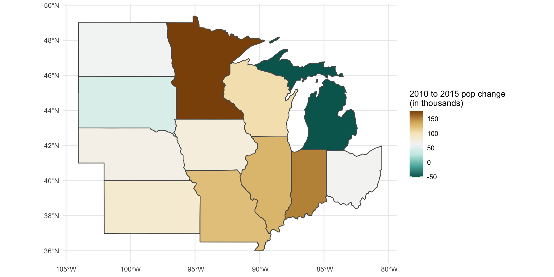
Pipes (%>% or |>) help make data transformation scripts easier to read and understand:

us_states %>%
  filter(REGION == "Midwest") %>%
  mutate(
    total_pop_change_10_15 = total_pop_change_10_15 / 1000
  )

Simple feature collection with 12 features and 8 fields
Geometry type: MULTIPOLYGON
Dimension:     XY
Bounding box:  xmin: -104.0577 ymin: 35.99568 xmax: -80.51869 ymax: 49.38436
Geodetic CRS:  NAD83
First 10 features:
   GEOID         NAME  REGION            AREA total_pop_10 total_pop_15
1     18      Indiana Midwest 36157.85 [mi^2]      6417398      6568645
2     20       Kansas Midwest 82254.08 [mi^2]      2809329      2892987
3     27    Minnesota Midwest 84388.99 [mi^2]      5241914      5419171
4     29     Missouri Midwest 69774.95 [mi^2]      5922314      6045448
5     38 North Dakota Midwest 70725.36 [mi^2]       659858       721640
6     46 South Dakota Midwest 77130.41 [mi^2]       799462       843190
7     17     Illinois Midwest 56368.25 [mi^2]     12745359     12873761
8     19         Iowa Midwest 56271.95 [mi^2]      3016267      3093526
9     26     Michigan Midwest 58347.38 [mi^2]      9952687      9900571
10    31     Nebraska Midwest 77325.58 [mi^2]      1799125      1869365
   total_pop_change_10_15                       geometry total_pop_10_scaled
1                 151.247 MULTIPOLYGON (((-87.52404 4...            6417.398
2                  83.658 MULTIPOLYGON (((-102.0517 4...            2809.329
3                 177.257 MULTIPOLYGON (((-97.22904 4...            5241.914
4                 123.134 MULTIPOLYGON (((-95.76565 4...            5922.314
5                  61.782 MULTIPOLYGON (((-104.0487 4...             659.858
6                  43.728 MULTIPOLYGON (((-104.0577 4...             799.462
7                 128.402 MULTIPOLYGON (((-91.41942 4...           12745.359
8                  77.259 MULTIPOLYGON (((-96.45326 4...            3016.267
9                 -52.116 MULTIPOLYGON (((-85.63002 4...            9952.687
10                 70.240 MULTIPOLYGON (((-104.0531 4...            1799.125

Tip: Packages to use with pipes

• {tidylog}
• {ViewPipeSteps}

Intermission: Maps and charts with {ggplot2}

The use of pipes is especially helpful with data visualizations where it reduces the need for intermediate placeholder objects or exports.

us_states %>%
  filter(REGION == "Midwest") %>%
  mutate(
    total_pop_change_10_15 = total_pop_change_10_15 / 1000
  ) %>%
  ggplot() +
  geom_sf(aes(fill = total_pop_change_10_15)) +
  scale_fill_distiller(type = "div") +
  labs(fill = "2010 to 2015 pop change\n(in thousands)")

Intermission: Maps and charts with {ggplot2}

You can also pass functions directly to the data and aesthetic arguments for {ggplot2} geoms:

ggplot(data = us_states %>% filter(REGION == "Midwest")) +
  geom_sf(aes(fill = total_pop_change_10_15 / 1000)) +
  scale_fill_distiller(type = "div") +
  labs(fill = "2010 to 2015 pop change\n(in thousands)")

us_states %>%
  arrange(desc(AREA)) %>%
  rename(Region = REGION) %>%
  slice_head(n = 10) %>%
  mutate(
    rank = row_number()
  ) %>%
  ggplot() +
  geom_sf(aes(fill = Region)) +
  geom_sf_label(aes(label = rank)) +
  scale_fill_brewer(type = "qual") +
  geom_sf(data = us_states, fill = NA) +
  labs(title = "10 largest states (by area) in U.S.")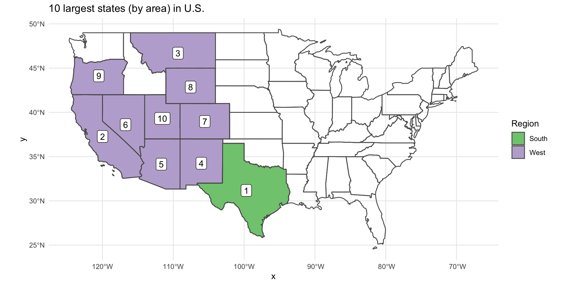

This example uses arrange() with a helper function desc() to sort by AREA in descending order, renames the REGION column to Region, subsets the first 10 rows with the slice_head() function, and add a rank label with mutate() and row_number functions. Note, that this example uses the scale_fill_brewer() scale function designed for discrete data (not continuous) and sets type = "qual" because region is a qualitative value with no ranking.

Additional topics

• using SQL queries to filter data
• {stringr} package and using regex
• using case_when() for recoding variables
• using pivot_longer() to pull variables from column names
• date and time variables

Recap on attribute data with R

• base R and dplyr both support many of the same tasks
• use pipes to chain together actions

References

Lovelace, Robin, Jakub Nowosad, and Jannes Muenchow. 2022. Geocomputation with R. 2nd (WIP). https://geocompr.robinlovelace.net/.