Mapping spatial data with R, ggplot2, and more

Overview

Working with spatial data using {sf} and {dplyr}
Mapping spatial data with {ggplot2}
Enhancing maps with extension packages

Working with spatial data using `{sf}` and `{dplyr}`

The sf package implements a simple features data model for vector spatial data in R
Vector geometries: points, lines, and polygons stored in a list-column of a data frame

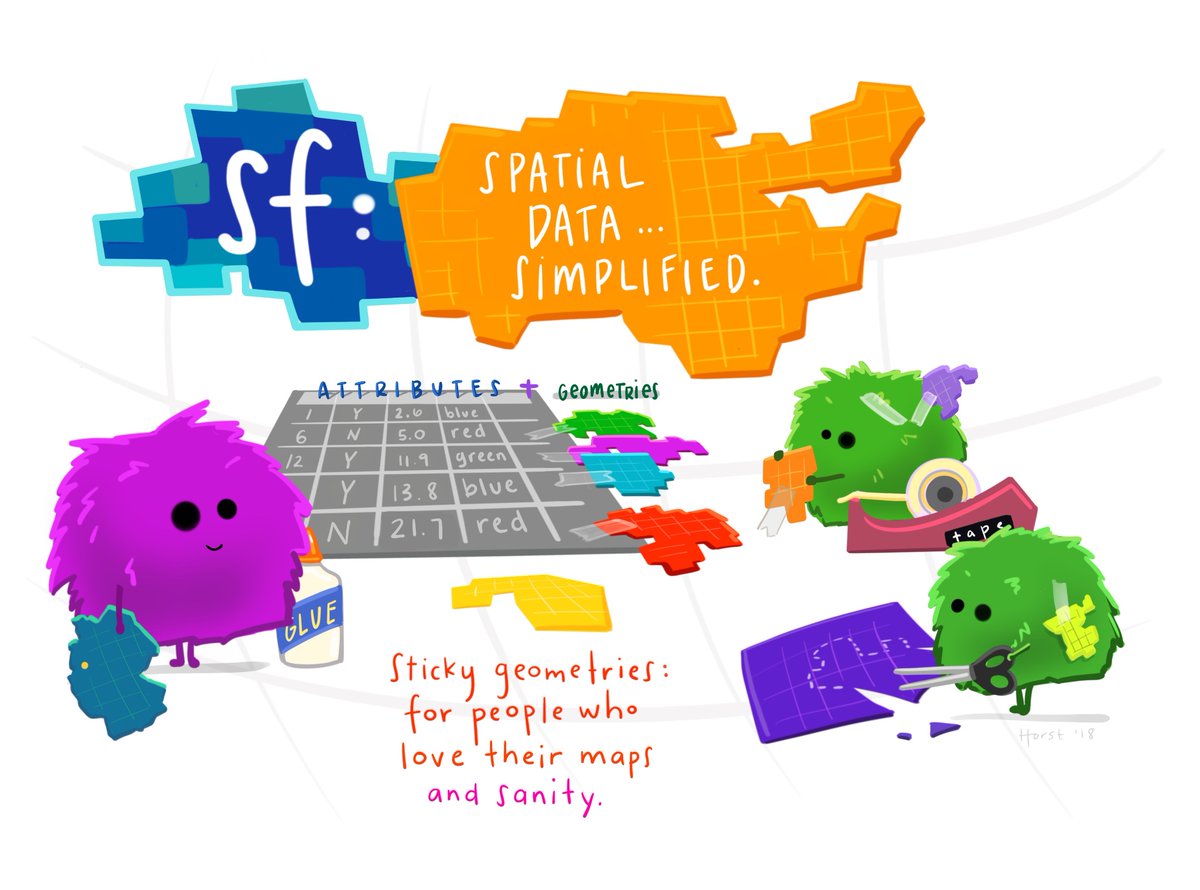
A simple feature (or sf) object is a data.frame with a “sticky” geometry column.

Reading data with `read_sf()`

Load the {sf} package and read a shapefile into your environment with read_sf():

library(sf)

nc <- read_sf(system.file("shape/nc.shp", package = "sf"))

Working with `sf` data.frames

You can subset columns and view a sf object just like any other data.frame in R:

nc[1:2, ]

Simple feature collection with 2 features and 14 fields
Geometry type: MULTIPOLYGON
Dimension:     XY
Bounding box:  xmin: -81.74107 ymin: 36.23436 xmax: -80.90344 ymax: 36.58965
Geodetic CRS:  NAD27
# A tibble: 2 × 15
   AREA PERIMETER CNTY_ CNTY_ID NAME   FIPS  FIPSNO CRESS_ID BIR74 SID74 NWBIR74
  <dbl>     <dbl> <dbl>   <dbl> <chr>  <chr>  <dbl>    <int> <dbl> <dbl>   <dbl>
1 0.114      1.44  1825    1825 Ashe   37009  37009        5  1091     1      10
2 0.061      1.23  1827    1827 Alleg… 37005  37005        3   487     0      10
# ℹ 4 more variables: BIR79 <dbl>, SID79 <dbl>, NWBIR79 <dbl>,
#   geometry <MULTIPOLYGON [°]>

Working with `sf` data.frames using `{dplyr}`

You can also use {dplyr} to sort a data.frame:

library(dplyr)

arrange(nc, desc(NAME))

Simple feature collection with 100 features and 14 fields
Geometry type: MULTIPOLYGON
Dimension:     XY
Bounding box:  xmin: -84.32385 ymin: 33.88199 xmax: -75.45698 ymax: 36.58965
Geodetic CRS:  NAD27
# A tibble: 100 × 15
    AREA PERIMETER CNTY_ CNTY_ID NAME  FIPS  FIPSNO CRESS_ID BIR74 SID74 NWBIR74
   <dbl>     <dbl> <dbl>   <dbl> <chr> <chr>  <dbl>    <int> <dbl> <dbl>   <dbl>
 1 0.08       1.31  1936    1936 Yanc… 37199  37199      100   770     0      12
 2 0.086      1.27  1893    1893 Yadk… 37197  37197       99  1269     1      65
 3 0.094      1.31  1979    1979 Wils… 37195  37195       98  3702    11    1827
 4 0.199      1.98  1874    1874 Wilk… 37193  37193       97  3146     4     200
 5 0.142      1.66  2029    2029 Wayne 37191  37191       96  6638    18    2593
 6 0.081      1.29  1880    1880 Wata… 37189  37189       95  1323     1      17
 7 0.1        1.33  1962    1962 Wash… 37187  37187       94   990     5     521
 8 0.118      1.42  1836    1836 Warr… 37185  37185       93   968     4     748
 9 0.219      2.13  1938    1938 Wake  37183  37183       92 14484    16    4397
10 0.072      1.08  1842    1842 Vance 37181  37181       91  2180     4    1179
# ℹ 90 more rows
# ℹ 4 more variables: BIR79 <dbl>, SID79 <dbl>, NWBIR79 <dbl>,
#   geometry <MULTIPOLYGON [°]>

Working with `sf` data.frames using `{dplyr}`

You can filter a data.frame by attributes:

filter(nc, AREA > 0.2)

Simple feature collection with 11 features and 14 fields
Geometry type: MULTIPOLYGON
Dimension:     XY
Bounding box:  xmin: -80.06441 ymin: 33.88199 xmax: -76.49254 ymax: 36.06665
Geodetic CRS:  NAD27
# A tibble: 11 × 15
    AREA PERIMETER CNTY_ CNTY_ID NAME  FIPS  FIPSNO CRESS_ID BIR74 SID74 NWBIR74
 * <dbl>     <dbl> <dbl>   <dbl> <chr> <chr>  <dbl>    <int> <dbl> <dbl>   <dbl>
 1 0.219      2.13  1938    1938 Wake  37183  37183       92 14484    16    4397
 2 0.201      1.80  1968    1968 Rand… 37151  37151       76  4456     7     384
 3 0.207      1.85  1989    1989 John… 37101  37101       51  3999     6    1165
 4 0.203      3.20  2004    2004 Beau… 37013  37013        7  2692     7    1131
 5 0.241      2.21  2083    2083 Samp… 37163  37163       82  3025     4    1396
 6 0.204      1.87  2100    2100 Dupl… 37061  37061       31  2483     4    1061
 7 0.24       2.00  2150    2150 Robe… 37155  37155       78  7889    31    5904
 8 0.225      2.11  2162    2162 Blad… 37017  37017        9  1782     8     818
 9 0.214      2.15  2185    2185 Pend… 37141  37141       71  1228     4     580
10 0.24       2.37  2232    2232 Colu… 37047  37047       24  3350    15    1431
11 0.212      2.02  2241    2241 Brun… 37019  37019       10  2181     5     659
# ℹ 4 more variables: BIR79 <dbl>, SID79 <dbl>, NWBIR79 <dbl>,
#   geometry <MULTIPOLYGON [°]>

What about the geometry – the spatial data?

The geometry column is a simple feature collection or sfc list column.

class(nc$geometry)

[1] "sfc_MULTIPOLYGON" "sfc"

What about the geometry – the spatial data?

A sfc object is a list of sfg or simple feature geometry objects.

class(nc$geometry[[1]])

[1] "XY"           "MULTIPOLYGON" "sfg"

Functions for working with `sf` geometry

The {sf} package provides a range of functions for exploring the geometry, coordinate reference system, bounding box, and other attributes of a simple feature object.

Functions for working with `sf` geometry

You can subset the geometry column:

nc$geometry

Geometry set for 100 features 
Geometry type: MULTIPOLYGON
Dimension:     XY
Bounding box:  xmin: -84.32385 ymin: 33.88199 xmax: -75.45698 ymax: 36.58965
Geodetic CRS:  NAD27
First 5 geometries:

Functions for working with `sf` geometry

You can check the geometry type with st_geometry_type():

st_geometry_type(nc, by_geometry = FALSE)

[1] MULTIPOLYGON
18 Levels: GEOMETRY POINT LINESTRING POLYGON MULTIPOINT ... TRIANGLE

Functions for working with `sf` geometry

You can look up the coordinate reference system with st_crs():

st_crs(nc)

Coordinate Reference System:
  User input: NAD27 
  wkt:
GEOGCRS["NAD27",
    DATUM["North American Datum 1927",
        ELLIPSOID["Clarke 1866",6378206.4,294.978698213898,
            LENGTHUNIT["metre",1]]],
    PRIMEM["Greenwich",0,
        ANGLEUNIT["degree",0.0174532925199433]],
    CS[ellipsoidal,2],
        AXIS["latitude",north,
            ORDER[1],
            ANGLEUNIT["degree",0.0174532925199433]],
        AXIS["longitude",east,
            ORDER[2],
            ANGLEUNIT["degree",0.0174532925199433]],
    ID["EPSG",4267]]

Functions for working with `sf` geometry

You can get a bounding box for the geometry with st_bbox():

st_bbox(nc)

     xmin      ymin      xmax      ymax 
-84.32385  33.88199 -75.45698  36.58965

Plotting `sf` objects

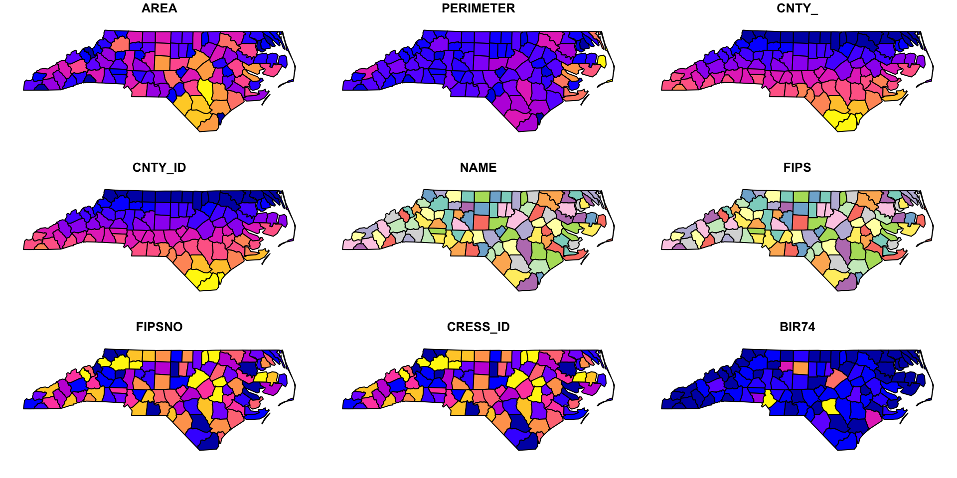
Of course, you probably want to see the geometry as well. You can use the built-in plot() method to make simple maps:

plot(nc)

Explore data interactively with `{mapview}`

You can also explore data interactively with {mapview}:

library(mapview)
mapview(nc)

Explore data interactively with `{mapview}`

Mapping spatial data with `{ggplot2}`

Before making a map {ggplot2}, we can start by downloading Maryland counties with the {tigris} package:

library(tigris)

md_counties <- counties(state = "MD", progress_bar = FALSE)
md_counties

Simple feature collection with 24 features and 17 fields
Geometry type: MULTIPOLYGON
Dimension:     XY
Bounding box:  xmin: -79.48765 ymin: 37.88661 xmax: -74.98628 ymax: 39.72304
Geodetic CRS:  NAD83
First 10 features:
     STATEFP COUNTYFP COUNTYNS GEOID         NAME            NAMELSAD LSAD
131       24      047 01668802 24047    Worcester    Worcester County   06
170       24      001 01713506 24001     Allegany     Allegany County   06
184       24      510 01702381 24510    Baltimore      Baltimore city   25
337       24      015 00596115 24015        Cecil        Cecil County   06
656       24      005 01695314 24005    Baltimore    Baltimore County   06
817       24      013 01696228 24013      Carroll      Carroll County   06
875       24      009 01676636 24009      Calvert      Calvert County   06
909       24      019 00596495 24019   Dorchester   Dorchester County   06
1026      24      003 01710958 24003 Anne Arundel Anne Arundel County   06
1051      24      021 01711211 24021    Frederick    Frederick County   06
     CLASSFP MTFCC CSAFP CBSAFP METDIVFP FUNCSTAT      ALAND     AWATER
131       H1 G4020   480  41540     <NA>        A 1213156434  586531107
170       H1 G4020  <NA>  19060     <NA>        A 1093489884   14710932
184       C7 G4020   548  12580     <NA>        F  209649327   28758743
337       H1 G4020   428  37980    48864        A  896912533  185281256
656       H1 G4020   548  12580     <NA>        A 1549740652  215957832
817       H1 G4020   548  12580     <NA>        A 1159355859   13112464
875       H1 G4020   548  47900    47894        A  552158542  341580668
909       H1 G4020   480  15700     <NA>        A 1400573746 1145353068
1026      H1 G4020   548  12580     <NA>        A 1074353889  448032843
1051      H1 G4020   548  47900    23224        A 1710922224   17674121
        INTPTLAT     INTPTLON                       geometry
131  +38.2221332 -075.3099315 MULTIPOLYGON (((-75.28336 3...
170  +39.6123134 -078.7031037 MULTIPOLYGON (((-78.80894 3...
184  +39.3000324 -076.6104761 MULTIPOLYGON (((-76.71151 3...
337  +39.5623537 -075.9415852 MULTIPOLYGON (((-75.77209 3...
656  +39.4431666 -076.6165693 MULTIPOLYGON (((-76.69766 3...
817  +39.5633280 -077.0153297 MULTIPOLYGON (((-76.95782 3...
875  +38.5227191 -076.5297621 MULTIPOLYGON (((-76.41579 3...
909  +38.4291957 -076.0474333 MULTIPOLYGON (((-75.913 38....
1026 +38.9916174 -076.5608941 MULTIPOLYGON (((-76.58029 3...
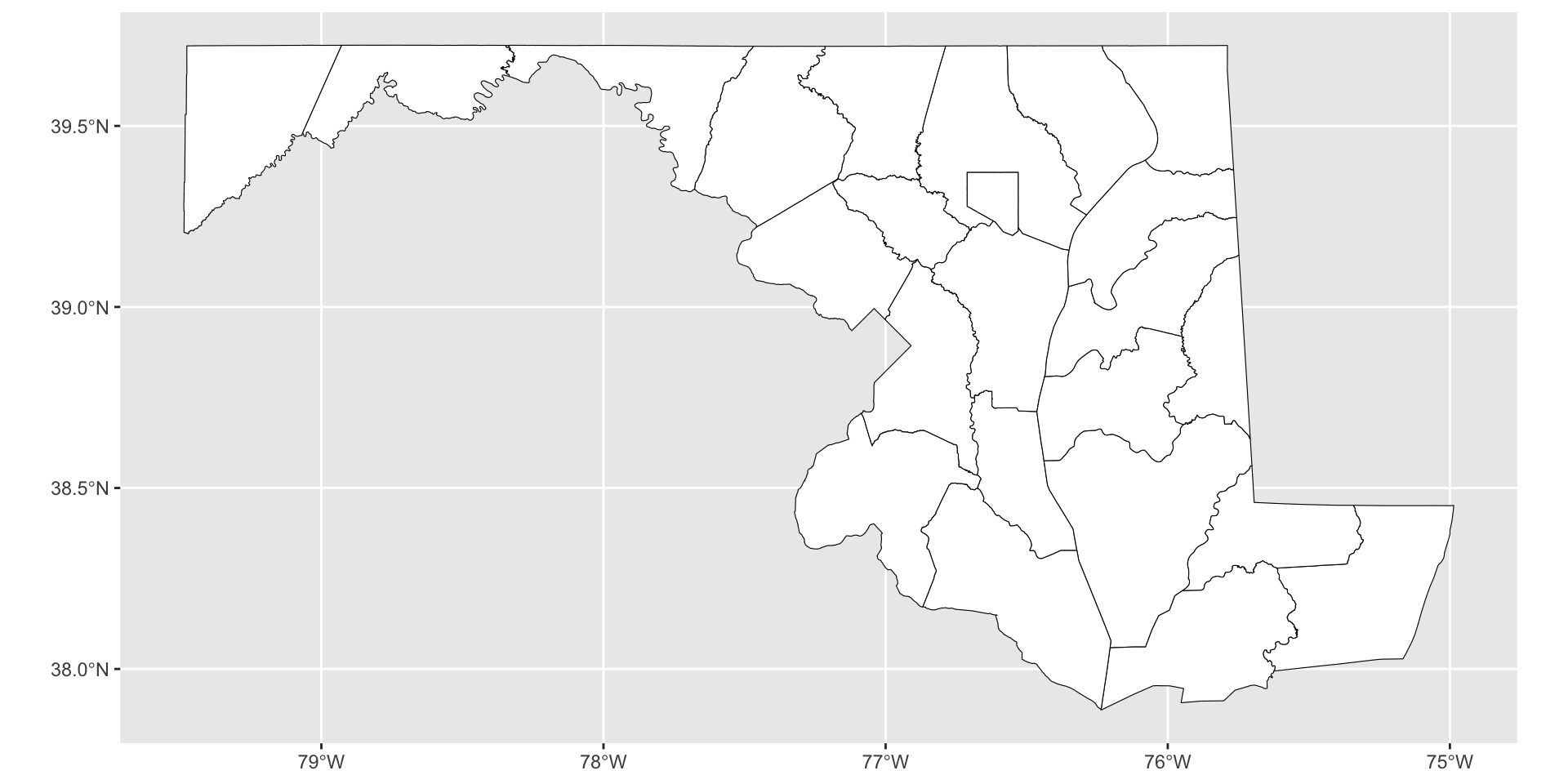
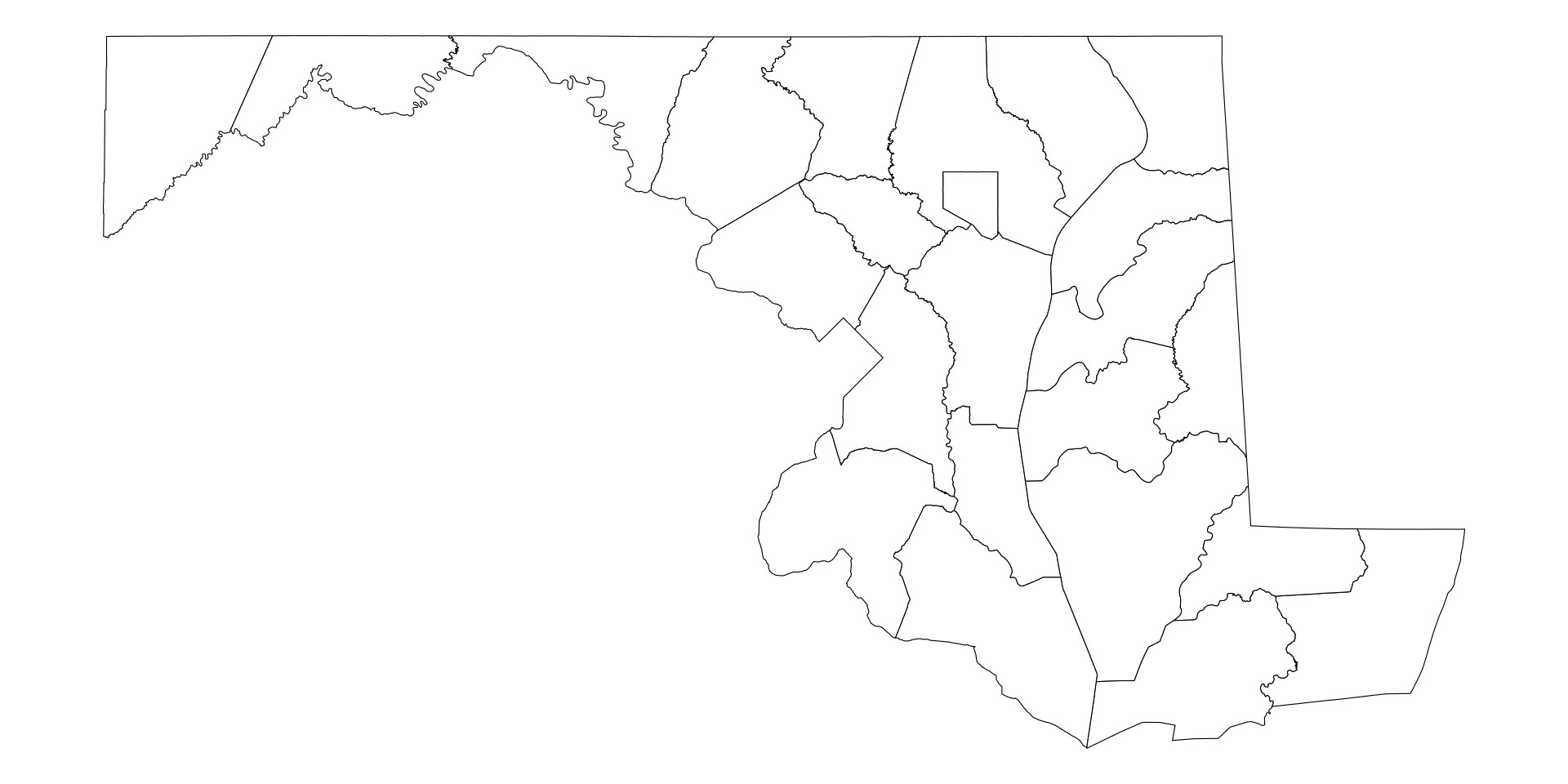
1051 +39.4701773 -077.3976358 MULTIPOLYGON (((-77.45475 3...

Creating a simple map with `{ggplot2}`

After loading the {ggplot2} package, making a map is as simple as supplying your data to ggplot() and adding a geom_sf() function:

library(ggplot2)

ggplot(data = md_counties) +
  geom_sf(
    color = "black",
    fill = "white"
  )

Creating a simple map with `{ggplot2}`

Adding a theme to a map

You can modify this map using a ggplot2 theme. theme_void(), for example, hides the graticules (grid lines) and axes:

ggplot(data = md_counties) +
  geom_sf(
    color = "black",
    fill = "white"
  ) +
  theme_void()

Adding a theme to a map

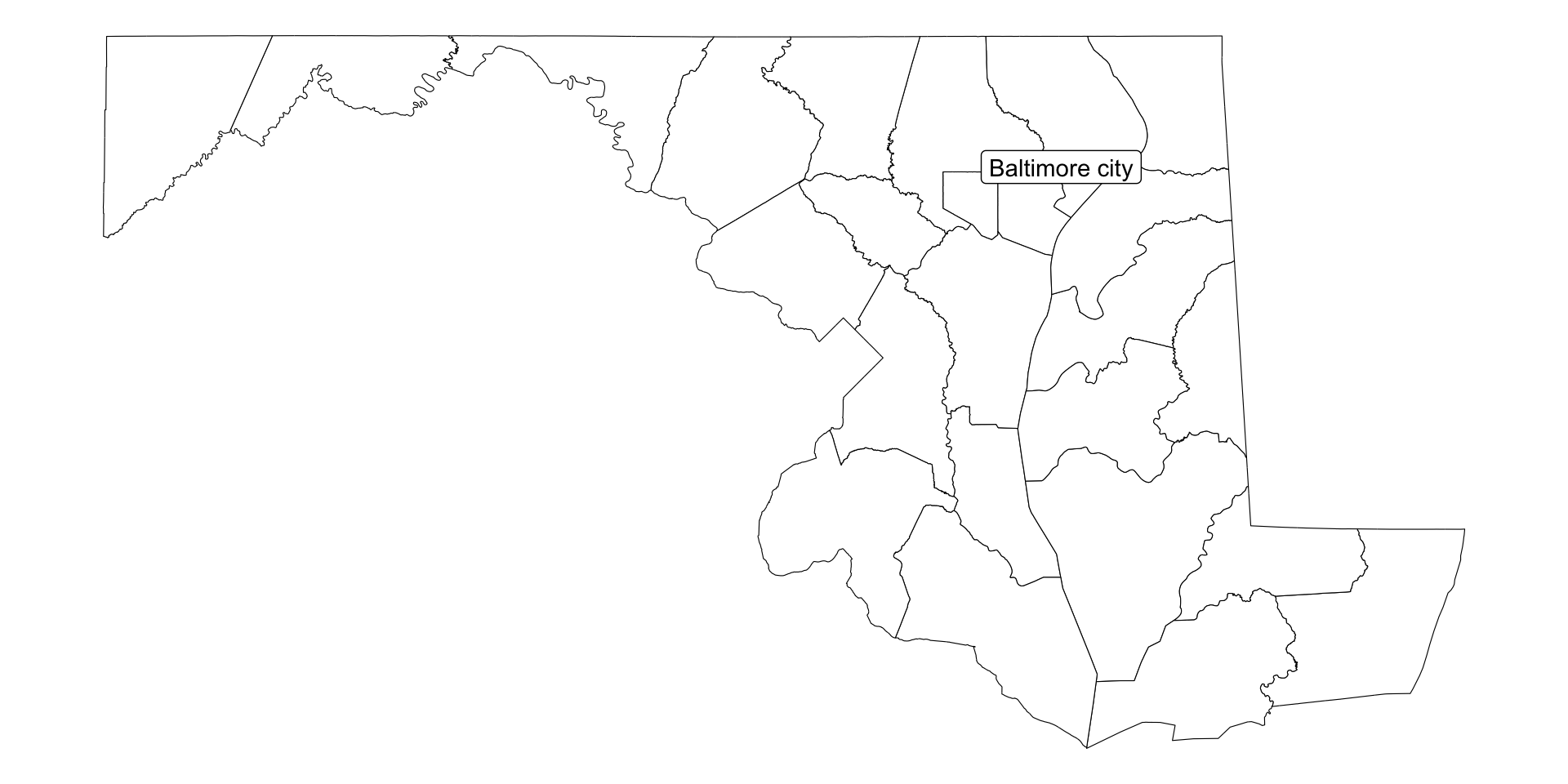
Adding text or labels to a map

You can add text with geom_sf_text() or a label with geom_sf_label() (using the nudge_x and nudge_y parameters to adjust label or text position):

ggplot(data = md_counties) +
  geom_sf(color = "black", fill = "white") +
  geom_sf_label(
    data = \(x) {
      filter(x, NAMELSAD == "Baltimore city")
    },
    mapping = aes(label = NAMELSAD),
    nudge_x = 0.3,
    nudge_y = 0.1
  ) +
  theme_void()

Adding text or labels to a map

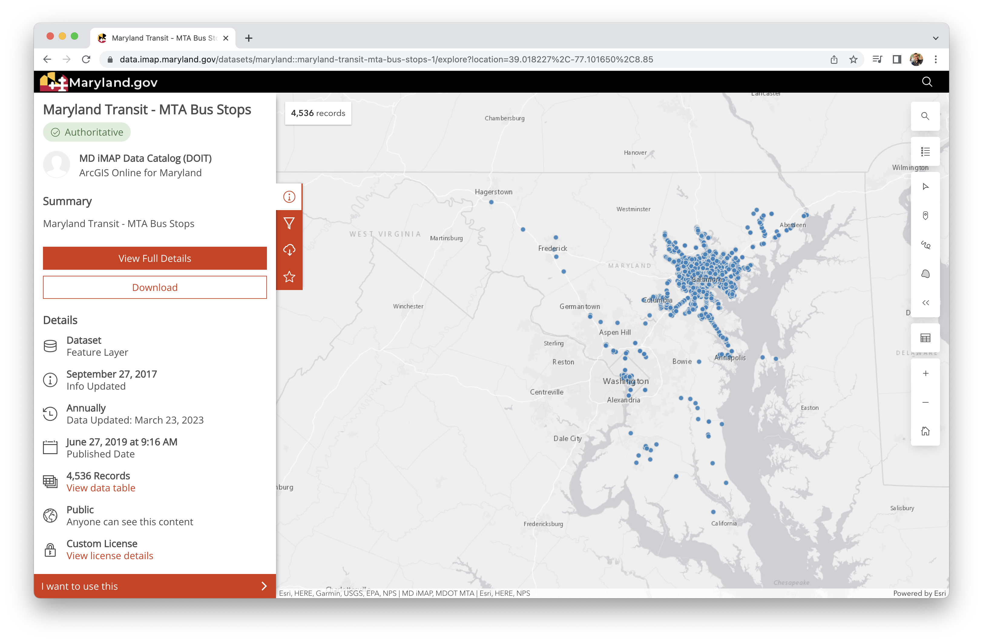
Reading data from Maryland iMap

I’ll use MTA bus stops for this workshop but pick a dataset that interests you.

Reading data from Maryland iMap

Find a GeoJSON URL and read with sf::read_sf():

mta_stops <- read_sf("https://geodata.md.gov/imap/rest/services/Transportation/MD_Transit/FeatureServer/9/query?outFields=*&where=1%3D1&f=geojson")

Explore data after reading with `dplyr::glimpse()`

Load dplyr and you can take a look at the object attributes with dplyr::glimpse():

glimpse(mta_stops)

Rows: 4,536
Columns: 13
$ OBJECTID            <int> 54570, 54571, 54572, 54573, 54574, 54575, 54576, 5…
$ stop_name           <chr> "CYLBURN AVE & GREENSPRING AVE fs wb", "LANIER AVE…
$ Rider_On            <int> 212, 34, 105, 31, 13, 4, 50, 47, 8, 0, 14, 6, 3, 1…
$ Rider_Off           <int> 172, 20, 18, 36, 24, 1, 21, 14, 6, 3, 12, 1, 12, 1…
$ Rider_Total         <int> 384, 54, 124, 67, 37, 5, 71, 61, 14, 3, 26, 8, 15,…
$ Stop_Ridership_Rank <int> 291, 2042, 1129, 1804, 2488, 3860, 1728, 1900, 339…
$ Routes_Served       <chr> "94, 31, 91", "94, 31, 91", "94, 31, 91", "91", "9…
$ Distribution_Policy <chr> "E1 - Public Domain - Internal Use Only", "E1 - Pu…
$ Mode                <chr> "Bus", "Bus", "Bus", "Bus", "Bus", "Bus", "Bus", "…
$ Shelter             <chr> "Yes", "No", "No", "No", "No", "No", "No", "No", "…
$ County              <chr> "Baltimore City", "Baltimore City", "Baltimore Cit…
$ stop_id             <chr> "1", "3", "4", "8", "10", "11", "12", "15", "16", …
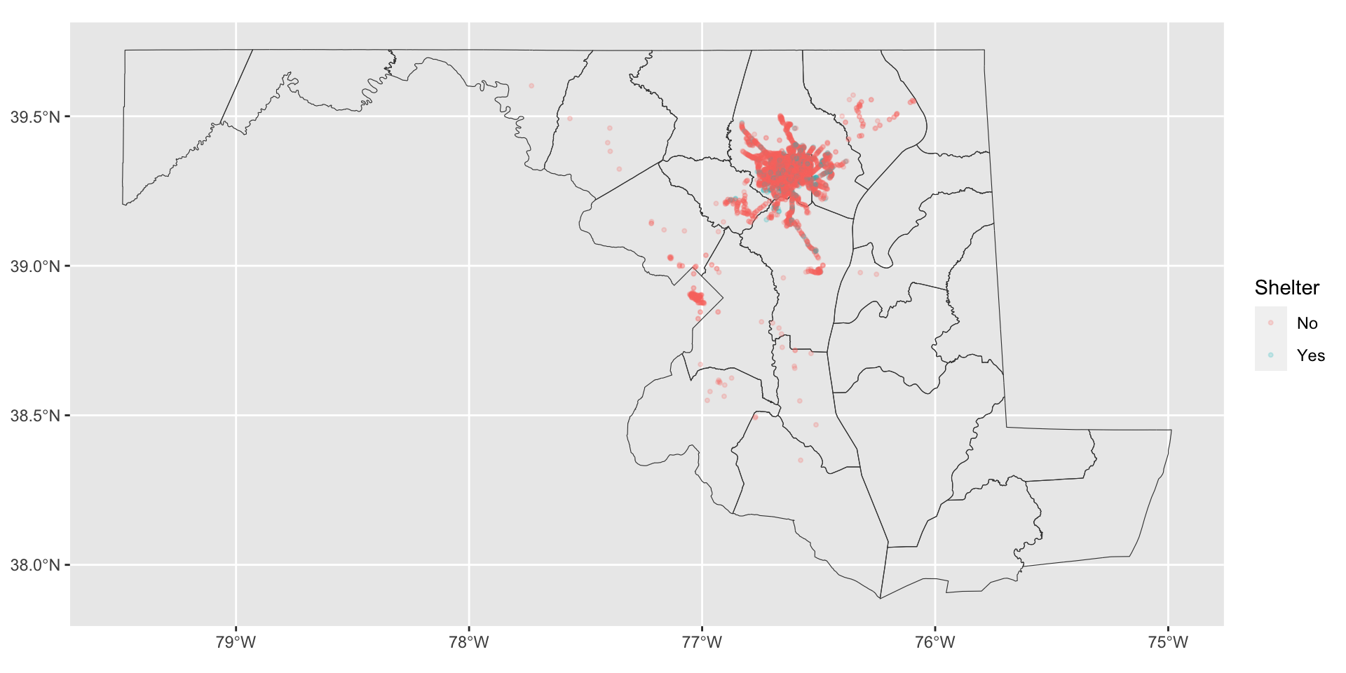
$ geometry            <POINT [°]> POINT (-76.66039 39.35095), POINT (-76.66336…

Map attributes to aesthetics using `aes()`

Make a map with md_counties and your additional data as a new layer:

ggplot(data = mta_stops) +
  geom_sf(data = md_counties, fill = NA, color = "gray25") +
  geom_sf(aes(color = Shelter), alpha = 0.2, size = 0.75)

Map attributes to aesthetics using `aes()`

🤔 Refining a map

This doesn’t look quite right yet. Let’s try out a few more changes:

Use ggplot2::coord_sf() to modify the map limits
Get roads and water from using tigris::roads() or tigris::area_water()
Apply a color scale from ColorBrewer using ggplot2::scale_color_brewer() or ggplot2::scale_color_distiller()
Limit stops to city using sf::st_crop() or sf::st_filter()

Use `coord_sf()` to modify the map limits

Filter Baltimore City from md_counties and convert the sf object into a bounding box (a bbox):

baltimore_city <- filter(md_counties, NAMELSAD == "Baltimore city")
baltimore_bbox <- st_bbox(baltimore_city)

Pass the xmin and xmax values from the bounding box to xlim and the ymin and ymax values from the bounding box to ylim:

baltimore_bbox_lims <- coord_sf(
  xlim = c(baltimore_bbox$xmin, baltimore_bbox$xmax),
  ylim = c(baltimore_bbox$ymin, baltimore_bbox$ymax)
)

Use `coord_sf()` to modify the map limits

mta_stop_map +
  baltimore_bbox_lims +
  theme_void()

Use `coord_sf()` to modify the map limits

Add roads and water from `{tigris}`

The tigris package is a helpful source for physical data as well as administrative data. For example, you can download roads and water areas:

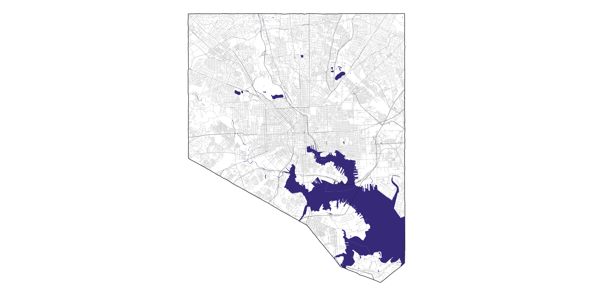
baltimore_roads <- roads(state = "MD", county = "Baltimore city")
baltimore_water <- area_water(state = "MD", county = "Baltimore city")

Combine layers into a list for reuse as a basemap

baltimore_layers <-
  list(
    geom_sf(data = baltimore_city, fill = "white", color = "black", linewidth = 0.25),
    geom_sf(data = baltimore_water, fill = "slateblue4", color = NA),
    geom_sf(data = baltimore_roads, color = "gray20", linewidth = 0.035),
    theme_void()
  )

baltimore_basemap <- ggplot() +
  baltimore_layers

baltimore_basemap

Combine layers into a list for reuse as a basemap

Apply a color scale from ColorBrewer

Start with the default colors:

baltimore_basemap +
  geom_sf(data = mta_stops, aes(color = Shelter), alpha = 0.35, size = 0.35) +
  baltimore_bbox_lims

Apply a color scale from ColorBrewer

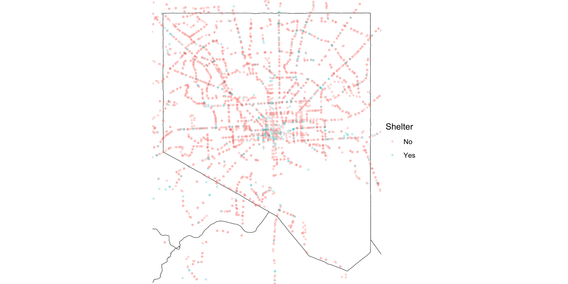
Set qualitative color scales with `scale_color_brewer()`

baltimore_basemap +
  geom_sf(
    data = mta_stops,
    aes(color = Shelter),
    alpha = 0.4, size = 0.6
  ) +
  baltimore_bbox_lims +
  scale_color_brewer(type = "qual", palette = "Dark2")

Set qualitative color scales with `scale_color_brewer()`

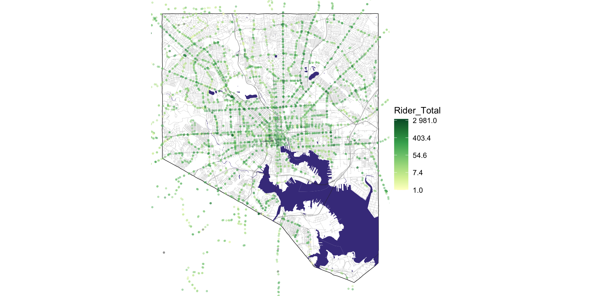
Set continuous color scales with `scale_color_distiller()`

baltimore_basemap +
  geom_sf(
    data = mta_stops,
    aes(color = Rider_Total),
    alpha = 0.4, size = 0.6
  ) +
  baltimore_bbox_lims +
  scale_color_distiller(
    palette = "YlGn",
    direction = 1, trans = "log",
    labels = scales::number
  )

Set continuous color scales with `scale_color_distiller()`

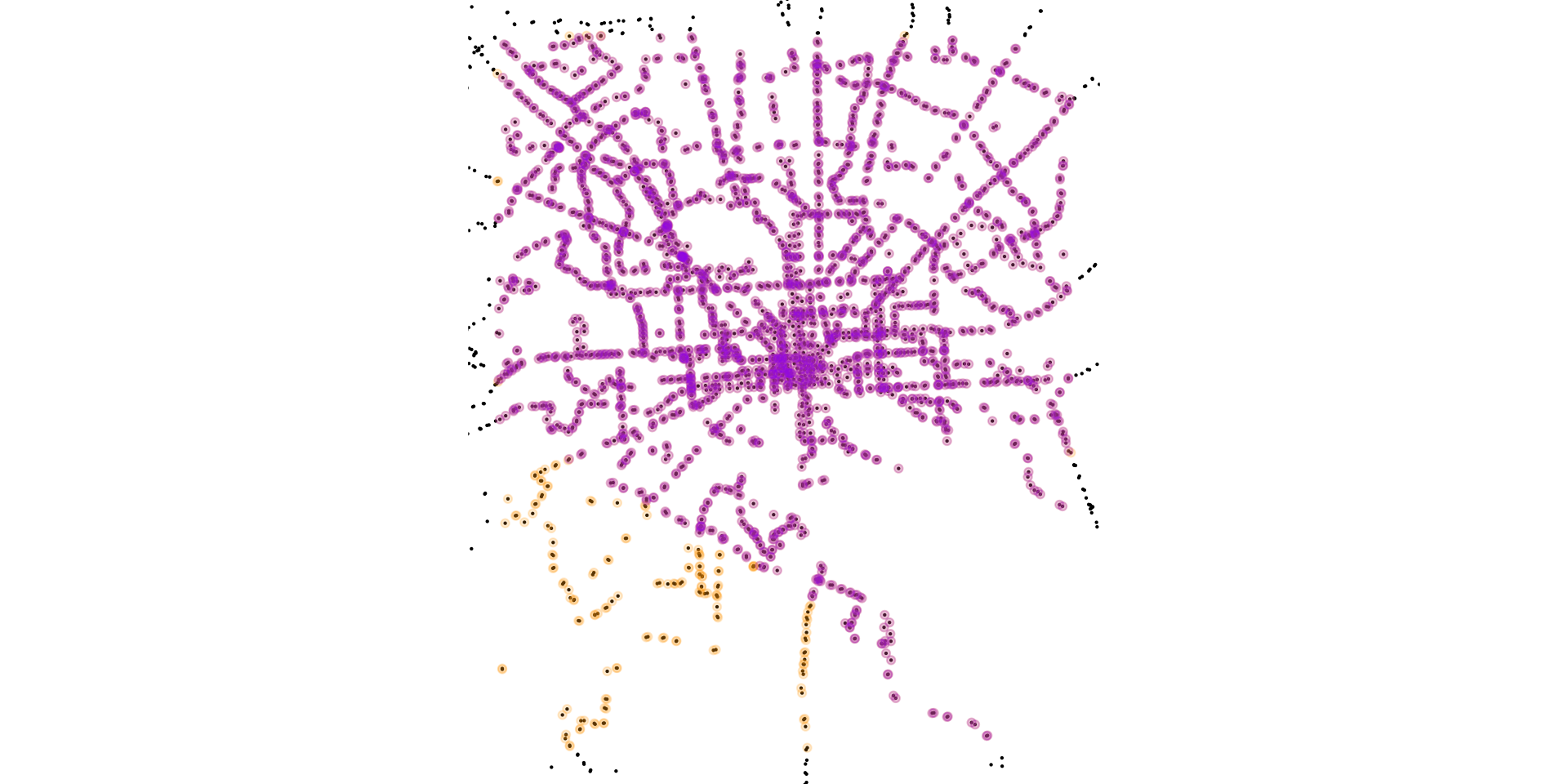
Use `st_crop()` or `st_filter()` to trim data to area

Match the coordinate reference system for two objects to crop or filter data:

mta_stops <- st_transform(mta_stops, 4269)

mta_stops_cropped <- st_crop(mta_stops, baltimore_bbox)

mta_stops_filtered <- st_filter(mta_stops, baltimore_city)

Compare the original stop data, stops cropped to Baltimore city’s bounding box, and stops filtered to Baltimore city’s geometry:

ggplot() +
  geom_sf(data = mta_stops, color = "black", size = 0.1) +
  geom_sf(data = mta_stops_cropped, color = "orange", alpha = 0.2) +
  geom_sf(data = mta_stops_filtered, color = "purple", alpha = 0.2) +
  baltimore_bbox_lims +
  theme_void()

You can also pass a list of objects to mapview to create layers and compare interactively:

mapview(list(mta_stops_cropped, mta_stops_filtered))

🎨 Refine maps using ggplot2 and extension packages

Use labs() to customize title and attribute labels
Label points with ggrepel::geom_text_repel()
Use basemaps from {mapboxapi}
Combine maps with {patchwork}

Adjust label positions with `ggrepel::geom_text_repel()`

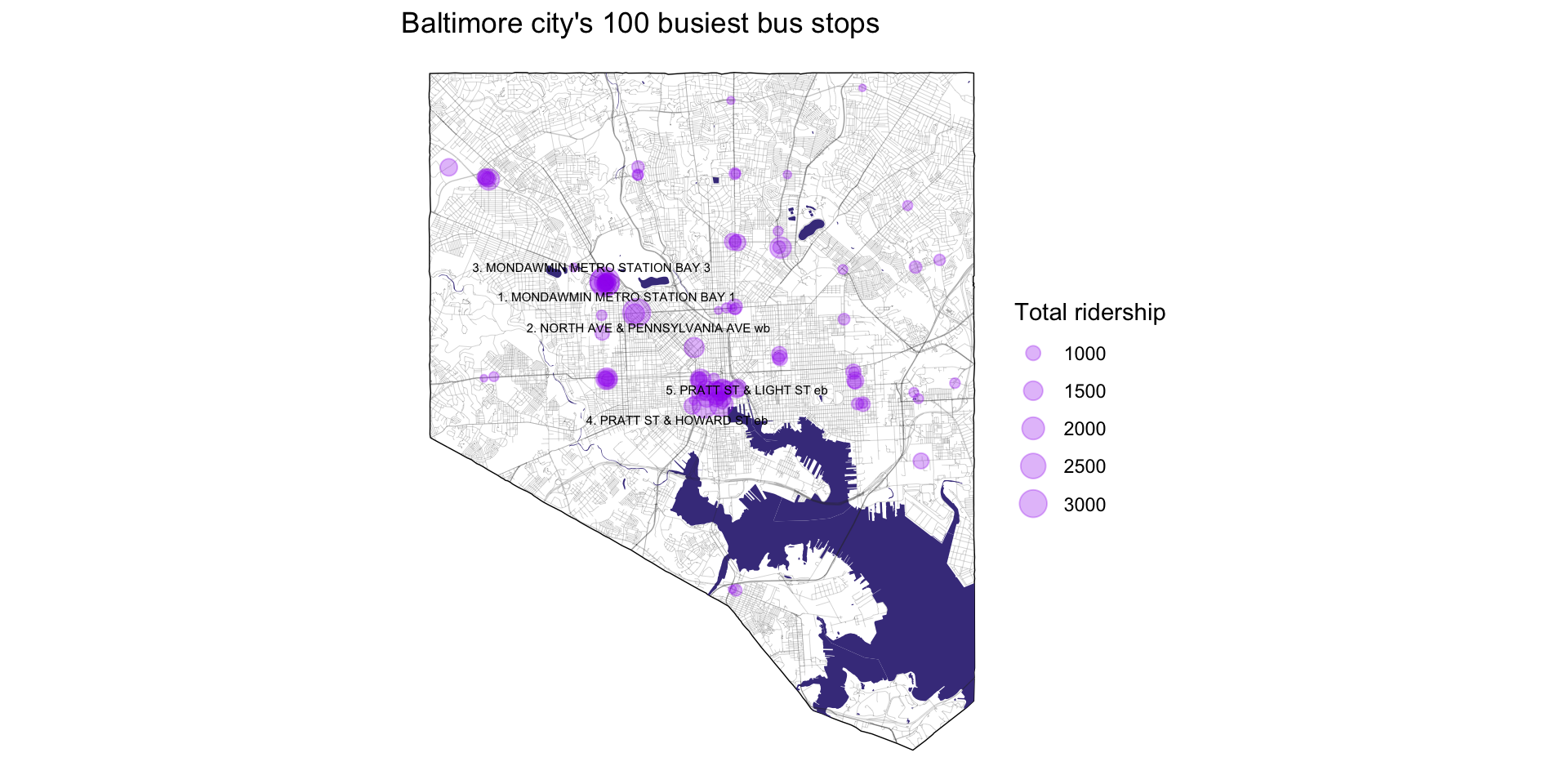
library(ggrepel)

baltimore_basemap +
  geom_sf(
    data = slice_max(mta_stops_filtered, order_by = desc(Stop_Ridership_Rank), n = 100),
    mapping = aes(size = Rider_Total),
    color = "purple", alpha = 0.3
  ) +
  geom_text_repel(
    data = slice_max(mta_stops_filtered, order_by = desc(Stop_Ridership_Rank), n = 5),
    aes(label = paste0(Stop_Ridership_Rank, ". ", stop_name), geometry = geometry),
    size = 2, stat = "sf_coordinates"
  ) +
  baltimore_bbox_lims +
  labs(
    title = "Baltimore city's 100 busiest bus stops",
    size = "Total ridership"
  )

Adjust label positions with `ggrepel::geom_text_repel()`

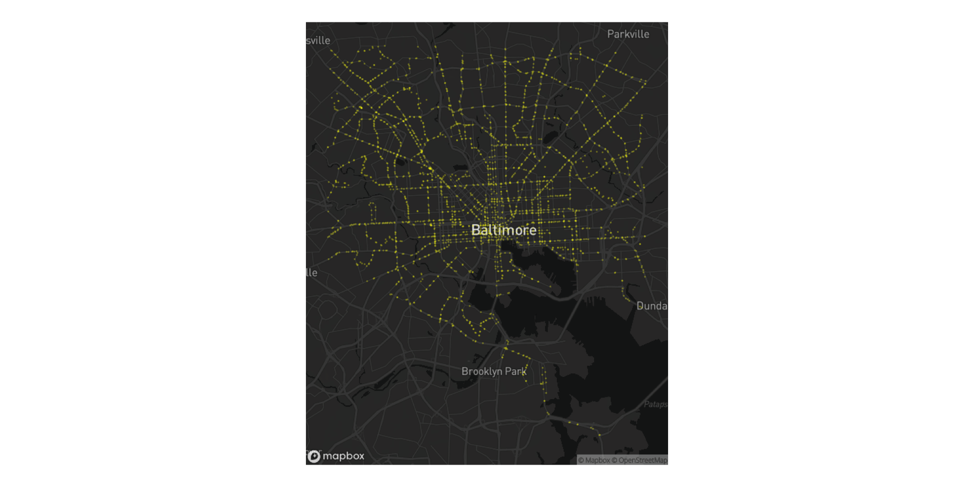
Use custom basemaps with `mapboxapi::layer_static_mapbox()`

library(mapboxapi)

mapbox_dark <-
  ggplot() +
  layer_static_mapbox(
    location = baltimore_city,
    style_url = "mapbox://styles/mapbox/dark-v10"
  ) +
  geom_sf(
    data = mta_stops_filtered,
    color = "yellow",
    alpha = 0.2,
    size = 0.05
  ) +
  theme_void()

mapbox_dark

Use custom basemaps with `mapboxapi::layer_static_mapbox()`

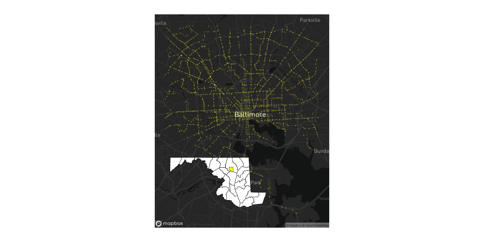
Add custom inset maps with `patchwork::inset_element()`

library(patchwork)

md_counties <- st_transform(md_counties, 3857)
baltimore_city <- st_transform(baltimore_city, 3857)

md_map <- ggplot() +
  geom_sf(data = md_counties, fill = "white", color = "black") +
  geom_sf(data = baltimore_city, fill = "yellow") +
  theme_void()

inset_md_map <-
  inset_element(
    md_map,
    left = 0.1,
    right = 0.65,
    top = 0.4,
    bottom = 0.075
  )

mapbox_dark + inset_md_map

Add custom inset maps with `patchwork::inset_element()`

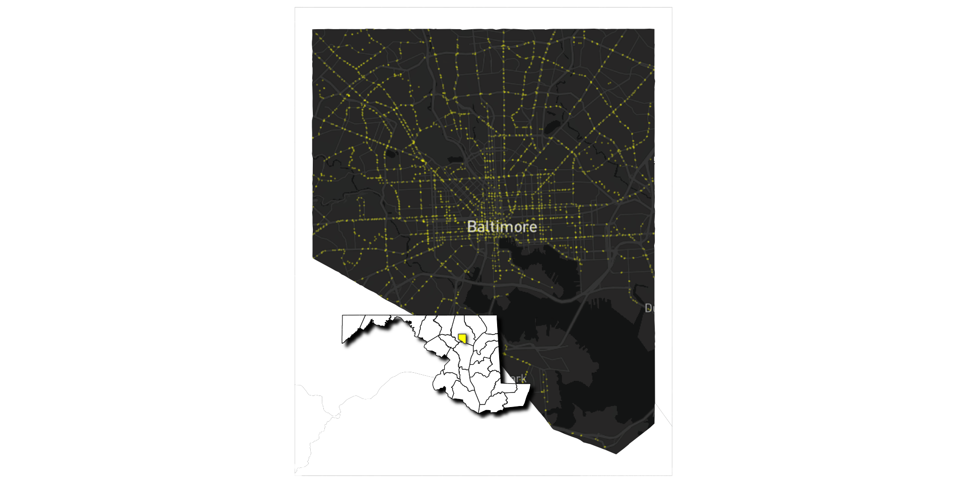
Add shadows with `ggfx::with_shadow()`

library(ggfx)

md_map <- ggplot() +
  with_shadow(
    geom_sf(data = md_counties, fill = "white", color = "black"),
    x_offset = 3,
    y_offset = 3
  ) +
  with_shadow(
    geom_sf(data = baltimore_city, fill = "yellow"),
    color = "gray20",
    x_offset = 1,
    y_offset = 1
  ) +
  theme_void()

md_map

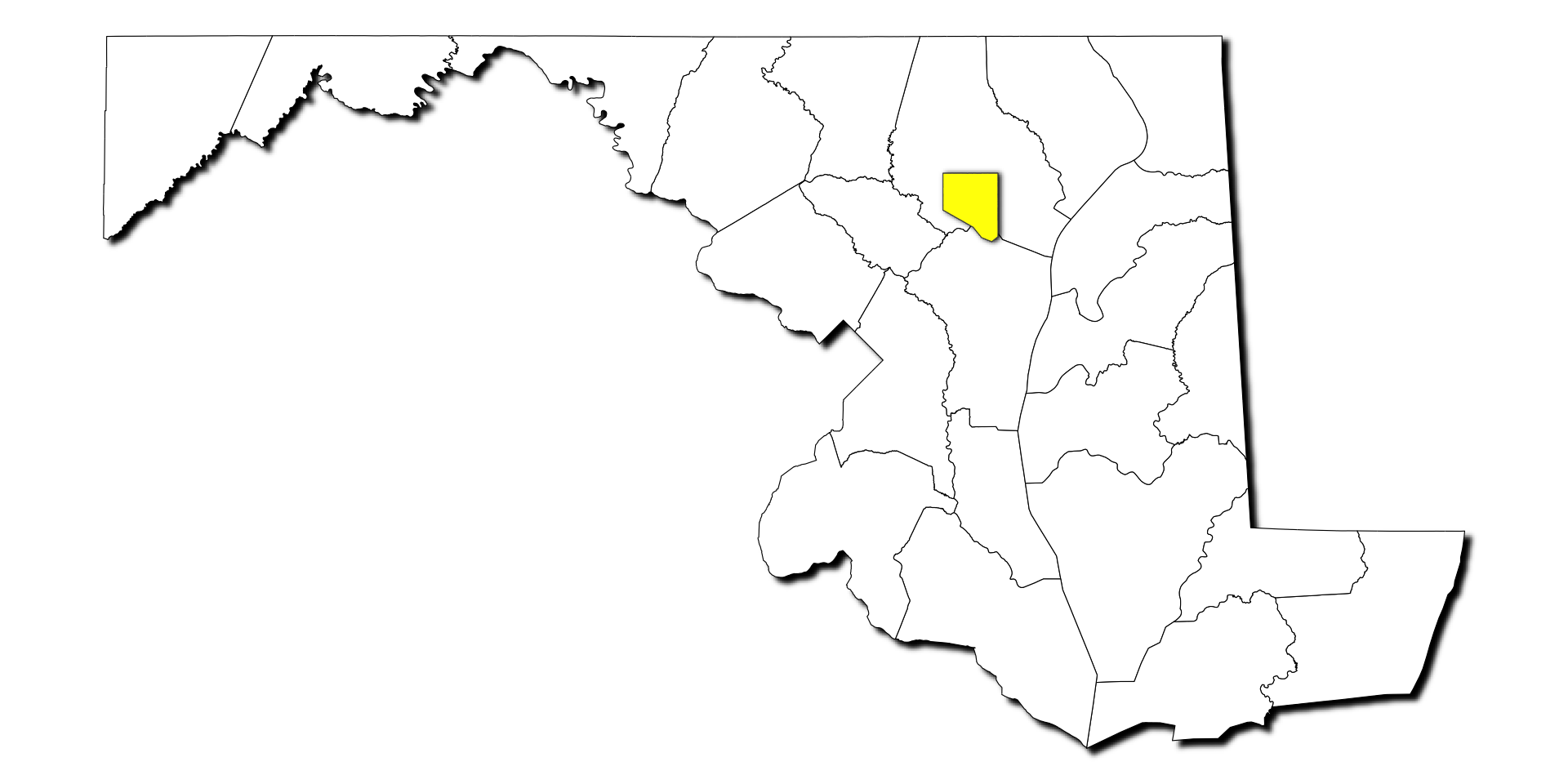
Add shadows with `ggfx::with_shadow()`

baltimore_bbox <- st_bbox(baltimore_city)

mapbox_dark +
  geom_sf(
    data = st_difference(md_counties, baltimore_city),
    fill = "white",
    alpha = 1,
    color = NA
  ) +
  coord_sf(
    xlim = c(baltimore_bbox$xmin, baltimore_bbox$xmax),
    ylim = c(baltimore_bbox$ymin, baltimore_bbox$ymax)
  ) +
  inset_element(
    md_map,
    left = 0.1,
    right = 0.65,
    top = 0.4,
    bottom = 0.075
  )

Add shadows with `ggfx::with_shadow()`

Convert static maps to interactive maps with {plotly}

md_counties_map <- ggplot() +
  geom_sf(data = md_counties, aes(fill = NAMELSAD))

plotly::ggplotly(md_counties_map)

Convert static maps to interactive maps with {plotly}

Resources

Essential R packages

sf
dplyr
ggplot2
scales
tmap (good alternative to ggplot2 for mapping)

Mapping spatial data with R, ggplot2, and more

Overview

Working with spatial data using {sf} and {dplyr}

Reading data with read_sf()

Working with sf data.frames

Working with sf data.frames using {dplyr}

Working with sf data.frames using {dplyr}

What about the geometry – the spatial data?

What about the geometry – the spatial data?

Functions for working with sf geometry

Functions for working with sf geometry

Functions for working with sf geometry

Functions for working with sf geometry

Functions for working with sf geometry

Plotting sf objects

Explore data interactively with {mapview}

Explore data interactively with {mapview}

Mapping spatial data with {ggplot2}

Creating a simple map with {ggplot2}

Creating a simple map with {ggplot2}

Adding a theme to a map

Adding a theme to a map

Adding text or labels to a map

Adding text or labels to a map

Reading data from Maryland iMap

Reading data from Maryland iMap

Reading data from Maryland iMap

Explore data after reading with dplyr::glimpse()

Map attributes to aesthetics using aes()

Map attributes to aesthetics using aes()

🤔 Refining a map

Use coord_sf() to modify the map limits

Use coord_sf() to modify the map limits

Use coord_sf() to modify the map limits

Add roads and water from {tigris}

Combine layers into a list for reuse as a basemap

Combine layers into a list for reuse as a basemap

Apply a color scale from ColorBrewer

Apply a color scale from ColorBrewer

Set qualitative color scales with scale_color_brewer()

Set qualitative color scales with scale_color_brewer()

Set continuous color scales with scale_color_distiller()

Set continuous color scales with scale_color_distiller()

Use st_crop() or st_filter() to trim data to area

🎨 Refine maps using ggplot2 and extension packages

Adjust label positions with ggrepel::geom_text_repel()

Adjust label positions with ggrepel::geom_text_repel()

Use custom basemaps with mapboxapi::layer_static_mapbox()

Use custom basemaps with mapboxapi::layer_static_mapbox()

Add custom inset maps with patchwork::inset_element()

Add custom inset maps with patchwork::inset_element()

Add shadows with ggfx::with_shadow()

Add shadows with ggfx::with_shadow()

Add shadows with ggfx::with_shadow()

Add shadows with ggfx::with_shadow()

Convert static maps to interactive maps with {plotly}

Convert static maps to interactive maps with {plotly}

Resources

Essential R packages

ggplot2 extension packages

Additional packages for spatial data

Working with spatial data using `{sf}` and `{dplyr}`

Reading data with `read_sf()`

Working with `sf` data.frames

Working with `sf` data.frames using `{dplyr}`

Working with `sf` data.frames using `{dplyr}`

Functions for working with `sf` geometry

Functions for working with `sf` geometry

Functions for working with `sf` geometry

Functions for working with `sf` geometry

Functions for working with `sf` geometry

Plotting `sf` objects

Explore data interactively with `{mapview}`

Explore data interactively with `{mapview}`

Mapping spatial data with `{ggplot2}`

Creating a simple map with `{ggplot2}`

Creating a simple map with `{ggplot2}`

Explore data after reading with `dplyr::glimpse()`

Map attributes to aesthetics using `aes()`

Map attributes to aesthetics using `aes()`

Use `coord_sf()` to modify the map limits

Use `coord_sf()` to modify the map limits

Use `coord_sf()` to modify the map limits

Add roads and water from `{tigris}`

Set qualitative color scales with `scale_color_brewer()`

Set qualitative color scales with `scale_color_brewer()`

Set continuous color scales with `scale_color_distiller()`

Set continuous color scales with `scale_color_distiller()`

Use `st_crop()` or `st_filter()` to trim data to area

Adjust label positions with `ggrepel::geom_text_repel()`

Adjust label positions with `ggrepel::geom_text_repel()`

Use custom basemaps with `mapboxapi::layer_static_mapbox()`

Use custom basemaps with `mapboxapi::layer_static_mapbox()`

Add custom inset maps with `patchwork::inset_element()`

Add custom inset maps with `patchwork::inset_element()`

Add shadows with `ggfx::with_shadow()`

Add shadows with `ggfx::with_shadow()`

Add shadows with `ggfx::with_shadow()`

Add shadows with `ggfx::with_shadow()`