The goal of getACS is to make it easier to work with American Community Survey data from the tidycensus package by Kyle Walker and others.
This package includes:
- Functions that extend
tidycensus::get_acs()to support multiple tables, geographies, or years - Functions for creating formatted tables from ACS data using the gt package
Note that I don’t love the current name for this package and expect to rename it as soon as I think of a better one.
Installation
You can install the development version of getACS from GitHub with:
# install.packages("pak")
pak::pkg_install("elipousson/getACS")
Usage
The main feature of getACS is support for returning multiple tables, geographies, and years.
acs_data <- get_acs_geographies(
  geography = c("county", "state"),
  county = "Baltimore city",
  state = "MD",
  table = "B08134",
  quiet = TRUE
)
The package also includes utility functions for filtering data and selecting columns to support the creation of tables using the gt package:
tbl_data <- filter_acs(acs_data, indent == 1, line_number <= 10)
tbl_data <- select_acs_cols(tbl_data)

commute_tbl <- gt_acs(
  tbl_data,
  groupname_col = "NAME",
  column_title_label = "Commute time",
  table = "B08134"
)

as_raw_html(commute_tbl)| Commute time | Est. | % share |
|---|---|---|
| Baltimore city, Maryland | ||
| Maryland | ||
| Source: 2017-2021 ACS 5-year Estimates, Table B08134. | ||
The gt_acs_compare() function also allows side-by-side comparison of geographies:
commute_tbl_compare <- gt_acs_compare(
  tbl_data,
  column_title_label = "Commute time",
  table = "B08134"
)

as_raw_html(commute_tbl_compare)| Est. | % share | Est. | % share | |
|---|---|---|---|---|
| Source: 2017-2021 ACS 5-year Estimates, Table B08134. | ||||
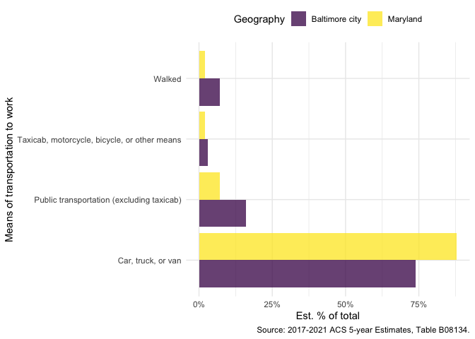
The package also includes several simple functions to support creating plots with the ggplot2 package:
plot_data <- filter_acs(acs_data, indent == 1, line_number > 10)
plot_data <- select_acs_cols(plot_data)

plot_data |>
  fmt_acs_county(state = "Maryland") |>
  ggplot(aes(x = perc_estimate, y = column_title, fill = NAME)) +
  geom_col(position = "dodge", alpha = 0.75) +
  scale_x_acs_percent() +
  scale_fill_viridis_d() +
  theme_minimal() +
  theme(legend.position = "top") +
  labs_acs_survey(
    y = "Means of transportation to work",
    fill = "Geography",
    table = acs_data$table_id
  )
For more information on working with Census data in R read the book Analyzing US Census Data: Methods, Maps, and Models in R (February 2023).
Related projects
Related R packages and analysis projects
- {easycensus}: Quickly Extract and Marginalize U.S. Census Tables
- {cwi}: Functions to speed up and standardize Census ACS data analysis for multiple staff people at DataHaven, preview trends and patterns, and get data in more layperson-friendly
- {camiller}: A set of convenience functions, functions for working with ACS data via tidycensus
- {psrccensus}: A set of tools developed for PSRC (Puget Sound Regional Council) staff to pull, process, and visualize Census Data for geographies in the Central Puget Sound Region.
- {CTPPr}: A R package for loading and working with the US Census CTPP survey data.
- {lehdr}: a package to grab LEHD data in support of city and regional planning economic and transportation analysis
- {mapreliability}: A R package for map classification reliability calculator
- Studying Neighborhoods With Uncertain Census Data: Code to create and visualize demographic clusters for the US with data from the American Community Survey
Related Python libraries
- census-data-aggregator: A Python library from the L.A. Times data desk to help “combine U.S. census data responsibly”
-
census-table-metadata: Tools for generating metadata about tables and fields in a Census release based on sequence lookup and table shell files. (Note: the pre-computed data from this repository is used to label ACS data by
label_acs_metadata())