1. Introduction to getACS

library(getACS)
library(dplyr)
library(ggplot2)
theme_set(theme_minimal())

This package is designed to build on the tidycensus package to make it easier to create reproducible reports by allowing users to:

• Download multiple tables with get_acs_tables()
• Download multiple geographies and tables with get_acs_geographies()
• Download multiple years and tables with get_acs_ts()

All of these functions use the label_acs_metadata() to join the variables to detailed pre-computed table and column metadata available on GitHub from the open-source Census Reporter project. This metadata includes a parent column ID that supports the conversion of estimate and margin of error values into a percent share of the corresponding total. The function also uses the race_iteration reference to add a name of the racial or ethnic group as a column where appropriate.

Using get_acs_tables()

Get the race iteration tables for a tenure status table using a county level geography:

tenure_tables <- acs_table_race_iteration("B25003")[c(2, 3, 10)]

tenure_data <- get_acs_tables(
  geography = "county",
  state = "MD",
  county = "Baltimore city",
  table = tenure_tables
)

Filter out the totals and create a simple bar chart to compare the data across tables:

tenure_data |>
  filter_acs(indent > 0) |>
  select_acs_cols("race_iteration_group") |>
  ggplot(aes(x = column_title, y = perc_estimate, fill = race_iteration_group)) +
  geom_col(alpha = 0.8, position = "dodge") +
  scale_y_acs_percent("% of households") +
  scale_fill_viridis_d("Race/ethnic group") +
  labs_acs_survey(table = tenure_tables, x = "Tenure")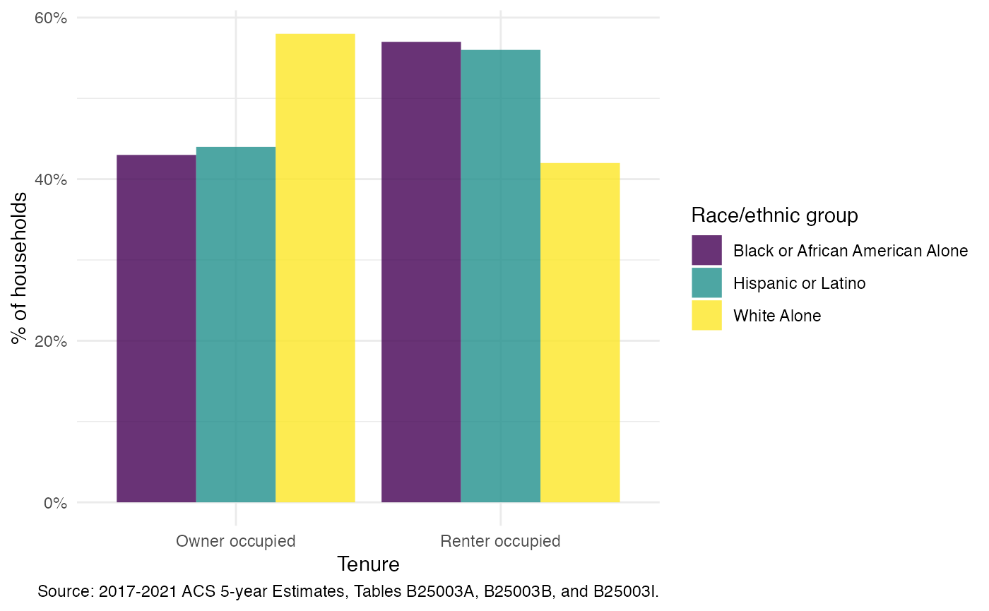

Using get_acs_geographies()

Get both county and state level geography for a population table:

multigeo_acs_data <- get_acs_geographies(
  geography = c("county", "state"),
  state = "MD",
  county = "Baltimore city",
  table = "B01003"
)

Drop the column title (the table contains only a single variable) and use the rowname_col parameter to group by the name of the area. fmt_acs_county() is a helper function to strip the text “, Maryland” from the end of the name of “Baltimore city”.

multigeo_acs_data |>
  select_acs_cols(column_title_col = NULL) |>
  gt_acs(
    rowname_col = "NAME",
    est_col_label = "Population"
  ) |>
  fmt_acs_county(state = "Maryland")

	Population
Baltimore city	592,211
Maryland	6,148,545
Source: 2017-2021 ACS 5-year Estimates.

Using get_acs_ts()

get_acs_ts() relies on a helper, acs_survey_ts(), that identifies the non-overlapping, comparable sample years for a specific ACS sample:

years <- acs_survey_ts("acs5", 2021)

years
#> [1] 2021 2016 2011

The get_acs_ts() calls acs_survey_ts() internally to return data for multiple years (warning you if a variable is unavailable for a specific year or geography):

acs_ts_data <- get_acs_ts(
  geography = "county",
  state = "MD",
  survey = "acs5",
  year = 2021,
  table = "B01003"
)

glimpse(acs_ts_data)
#> Rows: 72
#> Columns: 25
#> $ GEOID                    <chr> "24001", "24003", "24005", "24009", "24011", …
#> $ NAME                     <chr> "Allegany County, Maryland", "Anne Arundel Co…
#> $ variable                 <chr> "B01003_001", "B01003_001", "B01003_001", "B0…
#> $ column_id                <chr> "B01003001", "B01003001", "B01003001", "B0100…
#> $ table_id                 <chr> "B01003", "B01003", "B01003", "B01003", "B010…
#> $ estimate                 <dbl> 68684, 584064, 850702, 92515, 33234, 172148, …
#> $ moe                      <dbl> NA, NA, NA, NA, NA, NA, NA, NA, NA, NA, NA, N…
#> $ perc_estimate            <dbl> NA, NA, NA, NA, NA, NA, NA, NA, NA, NA, NA, N…
#> $ perc_moe                 <dbl> NA, NA, NA, NA, NA, NA, NA, NA, NA, NA, NA, N…
#> $ table_title              <chr> "Total Population", "Total Population", "Tota…
#> $ simple_table_title       <chr> "Total Population", "Total Population", "Tota…
#> $ subject_area             <chr> "Age-Sex", "Age-Sex", "Age-Sex", "Age-Sex", "…
#> $ universe                 <chr> "Total Population", "Total Population", "Tota…
#> $ denominator_column_id    <chr> NA, NA, NA, NA, NA, NA, NA, NA, NA, NA, NA, N…
#> $ topics                   <chr> "{\"age\",\"sex\"}", "{\"age\",\"sex\"}", "{\…
#> $ line_number              <dbl> 1, 1, 1, 1, 1, 1, 1, 1, 1, 1, 1, 1, 1, 1, 1, …
#> $ column_title             <chr> "Total", "Total", "Total", "Total", "Total", …
#> $ indent                   <dbl> 0, 0, 0, 0, 0, 0, 0, 0, 0, 0, 0, 0, 0, 0, 0, …
#> $ parent_column_id         <chr> NA, NA, NA, NA, NA, NA, NA, NA, NA, NA, NA, N…
#> $ denominator_estimate     <dbl> NA, NA, NA, NA, NA, NA, NA, NA, NA, NA, NA, N…
#> $ denominator_moe          <dbl> NA, NA, NA, NA, NA, NA, NA, NA, NA, NA, NA, N…
#> $ denominator_column_title <chr> NA, NA, NA, NA, NA, NA, NA, NA, NA, NA, NA, N…
#> $ geography                <chr> "county", "county", "county", "county", "coun…
#> $ state                    <chr> "MD", "MD", "MD", "MD", "MD", "MD", "MD", "MD…
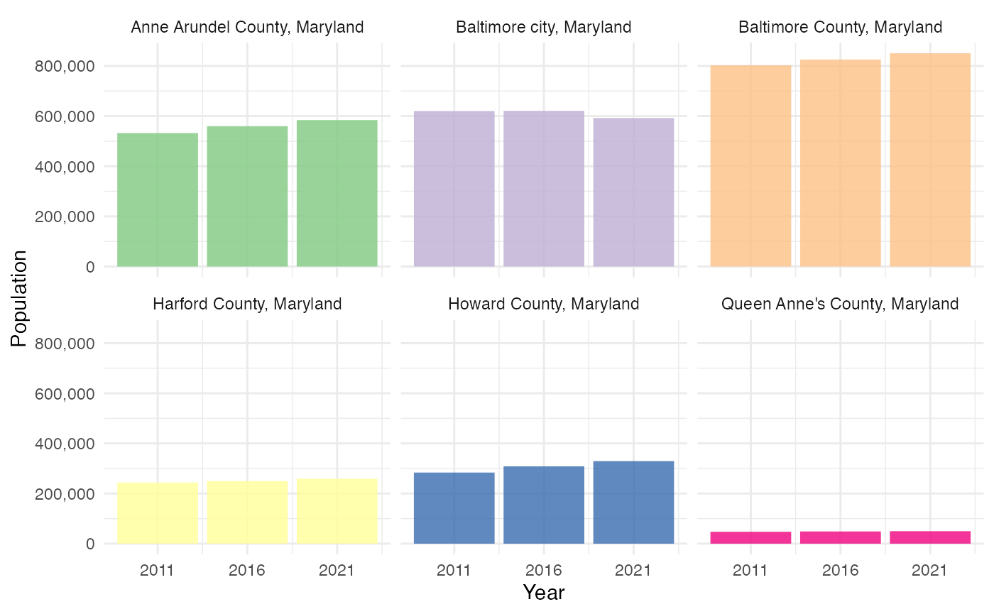
#> $ year                     <dbl> 2021, 2021, 2021, 2021, 2021, 2021, 2021, 202…

Helper functions for ggplot2 include scale_x_acs_ts() to set appropriate breaks:

acs_ts_data |>
  filter_acs(
    GEOID %in% c("24510", "24005", "24003", "24027", "24025", "24035")
  ) |>
  ggplot(aes(x = year, y = estimate, fill = NAME)) +
  geom_col(alpha = 0.8) +
  facet_wrap(~NAME) +
  scale_y_acs_estimate("Population") +
  scale_x_acs_ts(survey = "acs5", year = 2021) +
  scale_fill_brewer(type = "qual", guide = "none")