Read and filter spatial data with R

example

This example shows how to read spatial data into R using the sf package and explains the basic structure and attributes simple feature sf objects. This example uses two datasets from Natural Earth:

Admin 0 – Countries data (from 1:10m Cultural Vectors)
Populated Places (from 1:50m Cultural Vectors)

You are required to use this same data in completing the introductory assignments on reading and mapping data with QGIS and with R so this example.

Read spatial data

Tip

Review the sf vignette on Reading, Writing and Converting Simple Features for more detailed explanation on how to read spatial data into R.

Reading spatial data into your local R environment using the sf package is straight forward. For example, you can read a local GeoPackage file to an sf object by setting the dsn (short for data source name) to the file path:

dsn <- here::here("files/data", "ne_50m_populated_places_simple.gpkg")

populated_places <- st_read(dsn = dsn)

Reading layer `ne_50m_populated_places_simple' from data source 
  `/Users/elipousson/Documents/GitHub/bldgspatialdata/files/data/ne_50m_populated_places_simple.gpkg' 
  using driver `GPKG'
Simple feature collection with 1251 features and 31 fields
Geometry type: POINT
Dimension:     XY
Bounding box:  xmin: -175.2206 ymin: -90 xmax: 179.2166 ymax: 78.22097
Geodetic CRS:  WGS 84

st_read read the GeoPackage file into a simple feature (sf) object and output details on the layer, data source, driver, and attributes of the new object.

You can also use read_sf() which is the same as st_read() but it returns a tibble object and uses quiet = TRUE by default.

dsn <- here::here("files/data", "ne_10m_admin_0_countries.gpkg")

countries <- read_sf(dsn = dsn)

The dsn argument can also be a URL for a spatial data file that is stored online (instead of locally on your computer) or a database endpoint. The data source is also not limited to a GeoPackage files. Supported filetypes include GeoJSON files, shapefiles, KML files, and any other file type with a GDAL (Geospatial Data Abstraction Library) driver. You can review list available drivers using the sf::st_drivers() function.

Supported vector drivers
Supported raster drivers

Structure and attributes of sf objects

Tip

Read the sf vignette on Simple Features for R for more detailed explanation of geometry types, dimensions, coordinate reference systems, and more. For more on data frames, read the R Manual: An Introduction to R on data frames or the chapter on Tibbles from R for Data Science.

A simple feature (sf) object is always a data frame where each row is a feature. Like any other data frame, these columns can hold numeric (double or integer), character, factor, or logical values. These columns may also include list columns or nested data frame columns. The dplyr::glimpse() function provides a convenient way to get a quick overview of the column types and values for “populated_places” and “countries”:

glimpse(populated_places)

Rows: 1,251
Columns: 32
$ scalerank  <int> 10, 10, 10, 10, 10, 10, 10, 8, 8, 8, 8, 8, 7, 7, 7, 7, 7, 7…
$ natscale   <int> 1, 1, 1, 1, 1, 1, 1, 10, 10, 10, 10, 10, 20, 20, 20, 20, 20…
$ labelrank  <int> 5, 5, 3, 3, 3, 8, 0, 3, 3, 3, 3, 0, 6, 5, 5, 5, 5, 5, 5, 6,…
$ featurecla <chr> "Admin-1 region capital", "Admin-1 region capital", "Admin-…
$ name       <chr> "Bombo", "Fort Portal", "Potenza", "Campobasso", "Aosta", "…
$ namepar    <chr> NA, NA, NA, NA, NA, NA, NA, NA, NA, NA, NA, "Uruguay", NA, …
$ namealt    <chr> NA, NA, NA, NA, NA, NA, NA, NA, "Poitiers", NA, NA, NA, NA,…
$ nameascii  <chr> "Bombo", "Fort Portal", "Potenza", "Campobasso", "Aosta", "…
$ adm0cap    <int> 0, 0, 0, 0, 0, 0, 0, 1, 0, 0, 0, 0, 0, 0, 0, 0, 0, 0, 0, 0,…
$ capalt     <int> 0, 0, 0, 0, 0, 0, 0, 0, 0, 0, 0, 0, 0, 0, 0, 0, 0, 0, 0, 0,…
$ capin      <chr> NA, NA, NA, NA, NA, NA, NA, NA, NA, NA, NA, NA, NA, NA, NA,…
$ worldcity  <int> 0, 0, 0, 0, 0, 0, 0, 1, 0, 0, 0, 0, 0, 0, 0, 0, 0, 0, 0, 0,…
$ megacity   <int> 0, 0, 0, 0, 0, 0, 0, 0, 0, 0, 0, 0, 0, 0, 0, 0, 0, 0, 0, 0,…
$ sov0name   <chr> "Uganda", "Uganda", "Italy", "Italy", "Italy", "Finland", "…
$ sov_a3     <chr> "UGA", "UGA", "ITA", "ITA", "ITA", "ALD", "IS1", "VAT", "FR…
$ adm0name   <chr> "Uganda", "Uganda", "Italy", "Italy", "Italy", "Aland", "Pa…
$ adm0_a3    <chr> "UGA", "UGA", "ITA", "ITA", "ITA", "ALD", "PSX", "VAT", "FR…
$ adm1name   <chr> "Bamunanika", "Kabarole", "Basilicata", "Molise", "Valle d'…
$ iso_a2     <chr> "UG", "UG", "IT", "IT", "IT", "AX", "PS", "VA", "FR", "FR",…
$ note       <chr> NA, NA, NA, NA, NA, NA, NA, NA, NA, NA, NA, NA, NA, NA, NA,…
$ latitude   <dbl> 0.583299, 0.671004, 40.642002, 41.562999, 45.737001, 60.096…
$ longitude  <dbl> 32.533300, 30.275002, 15.798997, 14.655997, 7.315003, 19.94…
$ pop_max    <dbl> 75000, 42670, 69060, 50762, 34062, 10682, 24599, 832, 85960…
$ pop_min    <dbl> 21000, 42670, 69060, 50762, 34062, 10682, 24599, 832, 84807…
$ pop_other  <dbl> 0, 0, 0, 0, 0, 0, 0, 562430, 80866, 223592, 117010, 0, 7894…
$ rank_max   <int> 8, 7, 8, 8, 7, 6, 7, 2, 8, 10, 9, 1, 8, 10, 10, 10, 2, 8, 8…
$ rank_min   <int> 7, 7, 8, 8, 7, 6, 7, 2, 8, 9, 9, 1, 8, 8, 8, 8, 2, 8, 8, 7,…
$ meganame   <chr> NA, NA, NA, NA, NA, NA, NA, NA, NA, NA, NA, NA, NA, NA, NA,…
$ ls_name    <chr> NA, NA, NA, NA, NA, NA, NA, "Vatican City", "Poitier", "Cle…
$ min_zoom   <dbl> 7.0, 7.0, 7.0, 7.0, 7.0, 7.0, 9.0, 7.0, 6.7, 6.0, 7.0, 7.0,…
$ ne_id      <dbl> 1159113923, 1159113959, 1159117259, 1159117283, 1159117361,…
$ geom       <POINT [°]> POINT (32.5333 0.5832991), POINT (30.275 0.6710041), …

glimpse(countries)

Rows: 258
Columns: 169
$ featurecla <chr> "Admin-0 country", "Admin-0 country", "Admin-0 country", "A…
$ scalerank  <int> 0, 0, 0, 0, 0, 0, 3, 1, 0, 0, 0, 0, 0, 0, 0, 0, 0, 0, 0, 0,…
$ LABELRANK  <int> 2, 3, 2, 3, 2, 2, 3, 5, 2, 2, 4, 5, 5, 2, 3, 6, 2, 6, 3, 3,…
$ SOVEREIGNT <chr> "Indonesia", "Malaysia", "Chile", "Bolivia", "Peru", "Argen…
$ SOV_A3     <chr> "IDN", "MYS", "CHL", "BOL", "PER", "ARG", "GB1", "CYP", "IN…
$ ADM0_DIF   <int> 0, 0, 0, 0, 0, 0, 1, 0, 0, 1, 1, 1, 0, 0, 0, 0, 0, 0, 0, 0,…
$ LEVEL      <int> 2, 2, 2, 2, 2, 2, 2, 2, 2, 2, 2, 2, 2, 2, 2, 2, 2, 2, 2, 2,…
$ TYPE       <chr> "Sovereign country", "Sovereign country", "Sovereign countr…
$ TLC        <chr> "1", "1", "1", "1", "1", "1", "1", "1", "1", "1", "1", "1",…
$ ADMIN      <chr> "Indonesia", "Malaysia", "Chile", "Bolivia", "Peru", "Argen…
$ ADM0_A3    <chr> "IDN", "MYS", "CHL", "BOL", "PER", "ARG", "ESB", "CYP", "IN…
$ GEOU_DIF   <int> 0, 0, 0, 0, 0, 0, 0, 0, 0, 0, 0, 0, 0, 0, 0, 0, 0, 0, 0, 0,…
$ GEOUNIT    <chr> "Indonesia", "Malaysia", "Chile", "Bolivia", "Peru", "Argen…
$ GU_A3      <chr> "IDN", "MYS", "CHL", "BOL", "PER", "ARG", "ESB", "CYP", "IN…
$ SU_DIF     <int> 0, 0, 0, 0, 0, 0, 0, 0, 0, 0, 0, 0, 0, 0, 0, 0, 0, 0, 0, 0,…
$ SUBUNIT    <chr> "Indonesia", "Malaysia", "Chile", "Bolivia", "Peru", "Argen…
$ SU_A3      <chr> "IDN", "MYS", "CHL", "BOL", "PER", "ARG", "ESB", "CYP", "IN…
$ BRK_DIFF   <int> 0, 0, 0, 0, 0, 0, 0, 0, 0, 0, 1, 0, 0, 0, 0, 0, 0, 0, 0, 0,…
$ NAME       <chr> "Indonesia", "Malaysia", "Chile", "Bolivia", "Peru", "Argen…
$ NAME_LONG  <chr> "Indonesia", "Malaysia", "Chile", "Bolivia", "Peru", "Argen…
$ BRK_A3     <chr> "IDN", "MYS", "CHL", "BOL", "PER", "ARG", "ESB", "CYP", "IN…
$ BRK_NAME   <chr> "Indonesia", "Malaysia", "Chile", "Bolivia", "Peru", "Argen…
$ BRK_GROUP  <chr> NA, NA, NA, NA, NA, NA, NA, NA, NA, NA, NA, NA, NA, NA, NA,…
$ ABBREV     <chr> "Indo.", "Malay.", "Chile", "Bolivia", "Peru", "Arg.", "Dhe…
$ POSTAL     <chr> "INDO", "MY", "CL", "BO", "PE", "AR", "DH", "CY", "IND", "C…
$ FORMAL_EN  <chr> "Republic of Indonesia", "Malaysia", "Republic of Chile", "…
$ FORMAL_FR  <chr> NA, NA, NA, NA, NA, NA, NA, NA, NA, NA, NA, NA, NA, NA, NA,…
$ NAME_CIAWF <chr> "Indonesia", "Malaysia", "Chile", "Bolivia", "Peru", "Argen…
$ NOTE_ADM0  <chr> NA, NA, NA, NA, NA, NA, "U.K.", NA, NA, NA, NA, NA, NA, NA,…
$ NOTE_BRK   <chr> NA, NA, NA, NA, NA, NA, "U.K. Base", NA, NA, NA, NA, "Parti…
$ NAME_SORT  <chr> "Indonesia", "Malaysia", "Chile", "Bolivia", "Peru", "Argen…
$ NAME_ALT   <chr> NA, NA, NA, NA, NA, NA, NA, NA, NA, NA, NA, NA, NA, NA, NA,…
$ MAPCOLOR7  <int> 6, 2, 5, 1, 4, 3, 6, 1, 1, 4, 3, 3, 4, 4, 1, 2, 5, 1, 3, 2,…
$ MAPCOLOR8  <int> 6, 4, 1, 5, 4, 1, 6, 2, 3, 4, 2, 2, 4, 4, 3, 8, 2, 3, 6, 6,…
$ MAPCOLOR9  <int> 6, 3, 5, 2, 4, 3, 6, 3, 2, 4, 5, 5, 4, 1, 3, 6, 7, 4, 2, 2,…
$ MAPCOLOR13 <int> 11, 6, 9, 3, 11, 13, 3, 7, 2, 3, 9, 8, 12, 13, 5, 7, 3, 5, …
$ POP_EST    <dbl> 270625568, 31949777, 18952038, 11513100, 32510453, 44938712…
$ POP_RANK   <int> 17, 15, 14, 14, 15, 15, 5, 12, 18, 18, 13, 12, 13, 17, 14, …
$ POP_YEAR   <int> 2019, 2019, 2019, 2019, 2019, 2019, 2013, 2019, 2019, 2019,…
$ GDP_MD     <int> 1119190, 364681, 282318, 40895, 226848, 445445, 314, 24948,…
$ GDP_YEAR   <int> 2019, 2019, 2019, 2019, 2019, 2019, 2013, 2019, 2019, 2019,…
$ ECONOMY    <chr> "4. Emerging region: MIKT", "6. Developing region", "5. Eme…
$ INCOME_GRP <chr> "4. Lower middle income", "3. Upper middle income", "3. Upp…
$ FIPS_10    <chr> "ID", "MY", "CI", "BL", "PE", "AR", "-99", "CY", "IN", "CH"…
$ ISO_A2     <chr> "ID", "MY", "CL", "BO", "PE", "AR", "-99", "CY", "IN", "CN"…
$ ISO_A2_EH  <chr> "ID", "MY", "CL", "BO", "PE", "AR", "-99", "CY", "IN", "CN"…
$ ISO_A3     <chr> "IDN", "MYS", "CHL", "BOL", "PER", "ARG", "-99", "CYP", "IN…
$ ISO_A3_EH  <chr> "IDN", "MYS", "CHL", "BOL", "PER", "ARG", "-99", "CYP", "IN…
$ ISO_N3     <chr> "360", "458", "152", "068", "604", "032", "-99", "196", "35…
$ ISO_N3_EH  <chr> "360", "458", "152", "068", "604", "032", "-99", "196", "35…
$ UN_A3      <chr> "360", "458", "152", "068", "604", "032", "-099", "196", "3…
$ WB_A2      <chr> "ID", "MY", "CL", "BO", "PE", "AR", "-99", "CY", "IN", "CN"…
$ WB_A3      <chr> "IDN", "MYS", "CHL", "BOL", "PER", "ARG", "-99", "CYP", "IN…
$ WOE_ID     <int> 23424846, 23424901, 23424782, 23424762, 23424919, 23424747,…
$ WOE_ID_EH  <int> 23424846, 23424901, 23424782, 23424762, 23424919, 23424747,…
$ WOE_NOTE   <chr> "Exact WOE match as country", "Exact WOE match as country",…
$ ADM0_ISO   <chr> "IDN", "MYS", "CHL", "BOL", "PER", "ARG", "-99", "CYP", "IN…
$ ADM0_DIFF  <chr> NA, NA, NA, NA, NA, NA, "1", NA, NA, NA, NA, NA, NA, NA, "1…
$ ADM0_TLC   <chr> "IDN", "MYS", "CHL", "BOL", "PER", "ARG", "ESB", "CYP", "IN…
$ ADM0_A3_US <chr> "IDN", "MYS", "CHL", "BOL", "PER", "ARG", "ESB", "CYP", "IN…
$ ADM0_A3_FR <chr> "IDN", "MYS", "CHL", "BOL", "PER", "ARG", "ESB", "CYP", "IN…
$ ADM0_A3_RU <chr> "IDN", "MYS", "CHL", "BOL", "PER", "ARG", "ESB", "CYP", "IN…
$ ADM0_A3_ES <chr> "IDN", "MYS", "CHL", "BOL", "PER", "ARG", "ESB", "CYP", "IN…
$ ADM0_A3_CN <chr> "IDN", "MYS", "CHL", "BOL", "PER", "ARG", "ESB", "CYP", "IN…
$ ADM0_A3_TW <chr> "IDN", "MYS", "CHL", "BOL", "PER", "ARG", "ESB", "CYP", "IN…
$ ADM0_A3_IN <chr> "IDN", "MYS", "CHL", "BOL", "PER", "ARG", "ESB", "CYP", "IN…
$ ADM0_A3_NP <chr> "IDN", "MYS", "CHL", "BOL", "PER", "ARG", "ESB", "CYP", "IN…
$ ADM0_A3_PK <chr> "IDN", "MYS", "CHL", "BOL", "PER", "ARG", "ESB", "CYP", "IN…
$ ADM0_A3_DE <chr> "IDN", "MYS", "CHL", "BOL", "PER", "ARG", "ESB", "CYP", "IN…
$ ADM0_A3_GB <chr> "IDN", "MYS", "CHL", "BOL", "PER", "ARG", "ESB", "CYP", "IN…
$ ADM0_A3_BR <chr> "IDN", "MYS", "CHL", "BOL", "PER", "ARG", "ESB", "CYP", "IN…
$ ADM0_A3_IL <chr> "IDN", "MYS", "CHL", "BOL", "PER", "ARG", "ESB", "CYP", "IN…
$ ADM0_A3_PS <chr> "IDN", "MYS", "CHL", "BOL", "PER", "ARG", "ESB", "CYP", "IN…
$ ADM0_A3_SA <chr> "IDN", "MYS", "CHL", "BOL", "PER", "ARG", "ESB", "CYP", "IN…
$ ADM0_A3_EG <chr> "IDN", "MYS", "CHL", "BOL", "PER", "ARG", "ESB", "CYP", "IN…
$ ADM0_A3_MA <chr> "IDN", "MYS", "CHL", "BOL", "PER", "ARG", "ESB", "CYP", "IN…
$ ADM0_A3_PT <chr> "IDN", "MYS", "CHL", "BOL", "PER", "ARG", "ESB", "CYP", "IN…
$ ADM0_A3_AR <chr> "IDN", "MYS", "CHL", "BOL", "PER", "ARG", "ESB", "CYP", "IN…
$ ADM0_A3_JP <chr> "IDN", "MYS", "CHL", "BOL", "PER", "ARG", "ESB", "CYP", "IN…
$ ADM0_A3_KO <chr> "IDN", "MYS", "CHL", "BOL", "PER", "ARG", "ESB", "CYP", "IN…
$ ADM0_A3_VN <chr> "IDN", "MYS", "CHL", "BOL", "PER", "ARG", "ESB", "CYP", "IN…
$ ADM0_A3_TR <chr> "IDN", "MYS", "CHL", "BOL", "PER", "ARG", "ESB", "CYP", "IN…
$ ADM0_A3_ID <chr> "IDN", "MYS", "CHL", "BOL", "PER", "ARG", "ESB", "CYP", "IN…
$ ADM0_A3_PL <chr> "IDN", "MYS", "CHL", "BOL", "PER", "ARG", "ESB", "CYP", "IN…
$ ADM0_A3_GR <chr> "IDN", "MYS", "CHL", "BOL", "PER", "ARG", "ESB", "CYP", "IN…
$ ADM0_A3_IT <chr> "IDN", "MYS", "CHL", "BOL", "PER", "ARG", "ESB", "CYP", "IN…
$ ADM0_A3_NL <chr> "IDN", "MYS", "CHL", "BOL", "PER", "ARG", "ESB", "CYP", "IN…
$ ADM0_A3_SE <chr> "IDN", "MYS", "CHL", "BOL", "PER", "ARG", "ESB", "CYP", "IN…
$ ADM0_A3_BD <chr> "IDN", "MYS", "CHL", "BOL", "PER", "ARG", "ESB", "CYP", "IN…
$ ADM0_A3_UA <chr> "IDN", "MYS", "CHL", "BOL", "PER", "ARG", "ESB", "CYP", "IN…
$ ADM0_A3_UN <int> -99, -99, -99, -99, -99, -99, -99, -99, -99, -99, -99, -99,…
$ ADM0_A3_WB <int> -99, -99, -99, -99, -99, -99, -99, -99, -99, -99, -99, -99,…
$ CONTINENT  <chr> "Asia", "Asia", "South America", "South America", "South Am…
$ REGION_UN  <chr> "Asia", "Asia", "Americas", "Americas", "Americas", "Americ…
$ SUBREGION  <chr> "South-Eastern Asia", "South-Eastern Asia", "South America"…
$ REGION_WB  <chr> "East Asia & Pacific", "East Asia & Pacific", "Latin Americ…
$ NAME_LEN   <int> 9, 8, 5, 7, 4, 9, 8, 6, 5, 5, 6, 9, 7, 8, 8, 7, 5, 6, 8, 5,…
$ LONG_LEN   <int> 9, 8, 5, 7, 4, 9, 8, 6, 5, 5, 6, 9, 7, 8, 11, 7, 5, 6, 8, 5…
$ ABBREV_LEN <int> 5, 6, 5, 7, 4, 4, 5, 4, 5, 5, 4, 4, 4, 4, 7, 4, 4, 4, 5, 5,…
$ TINY       <int> -99, -99, -99, -99, -99, -99, 3, -99, -99, -99, -99, -99, 4…
$ HOMEPART   <int> 1, 1, 1, 1, 1, 1, -99, 1, 1, 1, 1, -99, 1, 1, 1, 1, 1, 1, 1…
$ MIN_ZOOM   <dbl> 0, 0, 0, 0, 0, 0, 0, 0, 0, 0, 0, 7, 0, 0, 0, 0, 0, 0, 0, 0,…
$ MIN_LABEL  <dbl> 1.7, 3.0, 1.7, 3.0, 2.0, 2.0, 6.5, 4.5, 1.7, 1.7, 3.0, 4.5,…
$ MAX_LABEL  <dbl> 6.7, 8.0, 6.7, 7.5, 7.0, 7.0, 11.0, 9.5, 6.7, 5.7, 8.0, 9.5…
$ LABEL_X    <dbl> 101.892949, 113.837080, -72.318871, -64.593433, -72.900160,…
$ LABEL_Y    <dbl> -0.954404, 2.528667, -38.151771, -16.666015, -12.976679, -3…
$ NE_ID      <dbl> 1159320845, 1159321083, 1159320493, 1159320439, 1159321163,…
$ WIKIDATAID <chr> "Q252", "Q833", "Q298", "Q750", "Q419", "Q414", "Q9206745",…
$ NAME_AR    <chr> "إندونيسيا", "ماليزيا", "تشيلي", "بوليفيا", "بيرو", "الأرجن…
$ NAME_BN    <chr> "ইন্দোনেশিয়া", "মালয়েশিয়া", "চিলি", "বলিভিয়া", "পেরু", "আর্জেন্…
$ NAME_DE    <chr> "Indonesien", "Malaysia", "Chile", "Bolivien", "Peru", "Arg…
$ NAME_EN    <chr> "Indonesia", "Malaysia", "Chile", "Bolivia", "Peru", "Argen…
$ NAME_ES    <chr> "Indonesia", "Malasia", "Chile", "Bolivia", "Perú", "Argent…
$ NAME_FA    <chr> "اندونزی", "مالزی", "شیلی", "بولیوی", "پرو", "آرژانتین", "د…
$ NAME_FR    <chr> "Indonésie", "Malaisie", "Chili", "Bolivie", "Pérou", "Arge…
$ NAME_EL    <chr> "Ινδονησία", "Μαλαισία", "Χιλή", "Βολιβία", "Περού", "Αργεν…
$ NAME_HE    <chr> "אינדונזיה", "מלזיה", "צ'ילה", "בוליביה", "פרו", "ארגנטינה"…
$ NAME_HI    <chr> "इंडोनेशिया", "मलेशिया", "चिली", "बोलिविया", "पेरू", "अर्जेण्टीना",…
$ NAME_HU    <chr> "Indonézia", "Malajzia", "Chile", "Bolívia", "Peru", "Argen…
$ NAME_ID    <chr> "Indonesia", "Malaysia", "Chili", "Bolivia", "Peru", "Argen…
$ NAME_IT    <chr> "Indonesia", "Malaysia", "Cile", "Bolivia", "Perù", "Argent…
$ NAME_JA    <chr> "インドネシア", "マレーシア", "チリ", "ボリビア", "ペルー",…
$ NAME_KO    <chr> "인도네시아", "말레이시아", "칠레", "볼리비아", "페루", "아…
$ NAME_NL    <chr> "Indonesië", "Maleisië", "Chili", "Bolivia", "Peru", "Argen…
$ NAME_PL    <chr> "Indonezja", "Malezja", "Chile", "Boliwia", "Peru", "Argent…
$ NAME_PT    <chr> "Indonésia", "Malásia", "Chile", "Bolívia", "Peru", "Argent…
$ NAME_RU    <chr> "Индонезия", "Малайзия", "Чили", "Боливия", "Перу", "Аргент…
$ NAME_SV    <chr> "Indonesien", "Malaysia", "Chile", "Bolivia", "Peru", "Arge…
$ NAME_TR    <chr> "Endonezya", "Malezya", "Şili", "Bolivya", "Peru", "Arjanti…
$ NAME_UK    <chr> "Індонезія", "Малайзія", "Чилі", "Болівія", "Перу", "Аргент…
$ NAME_UR    <chr> "انڈونیشیا", "ملائیشیا", "چلی", "بولیویا", "پیرو", "ارجنٹائ…
$ NAME_VI    <chr> "Indonesia", "Malaysia", "Chile", "Bolivia", "Peru", "Argen…
$ NAME_ZH    <chr> "印度尼西亚", "马来西亚", "智利", "玻利维亚", "秘鲁", "阿根…
$ NAME_ZHT   <chr> "印度尼西亞", "馬來西亞", "智利", "玻利維亞", "秘魯", "阿根…
$ FCLASS_ISO <chr> "Admin-0 country", "Admin-0 country", "Admin-0 country", "A…
$ TLC_DIFF   <chr> NA, NA, NA, NA, NA, NA, "1", NA, NA, NA, NA, NA, NA, NA, NA…
$ FCLASS_TLC <chr> "Admin-0 country", "Admin-0 country", "Admin-0 country", "A…
$ FCLASS_US  <chr> NA, NA, NA, NA, NA, NA, "Admin-0 dependency", NA, NA, NA, N…
$ FCLASS_FR  <chr> NA, NA, NA, NA, NA, NA, "Admin-0 dependency", NA, NA, NA, N…
$ FCLASS_RU  <chr> NA, NA, NA, NA, NA, NA, NA, NA, NA, NA, NA, NA, NA, NA, NA,…
$ FCLASS_ES  <chr> NA, NA, NA, NA, NA, NA, "Admin-0 dependency", NA, NA, NA, N…
$ FCLASS_CN  <chr> NA, NA, NA, NA, NA, NA, NA, NA, NA, NA, NA, NA, NA, NA, NA,…
$ FCLASS_TW  <chr> NA, NA, NA, NA, NA, NA, NA, NA, NA, "Unrecognized", NA, NA,…
$ FCLASS_IN  <chr> NA, NA, NA, NA, NA, NA, NA, NA, NA, NA, NA, NA, NA, NA, NA,…
$ FCLASS_NP  <chr> NA, NA, NA, NA, NA, NA, NA, NA, NA, NA, NA, NA, NA, NA, NA,…
$ FCLASS_PK  <chr> NA, NA, NA, NA, NA, NA, NA, NA, NA, NA, "Unrecognized", "Ad…
$ FCLASS_DE  <chr> NA, NA, NA, NA, NA, NA, "Admin-0 dependency", NA, NA, NA, N…
$ FCLASS_GB  <chr> NA, NA, NA, NA, NA, NA, "Admin-0 dependency", NA, NA, NA, N…
$ FCLASS_BR  <chr> NA, NA, NA, NA, NA, NA, NA, NA, NA, NA, NA, NA, NA, NA, NA,…
$ FCLASS_IL  <chr> NA, NA, NA, NA, NA, NA, NA, NA, NA, NA, NA, NA, NA, NA, NA,…
$ FCLASS_PS  <chr> NA, NA, NA, NA, NA, NA, NA, NA, NA, NA, NA, "Admin-0 countr…
$ FCLASS_SA  <chr> NA, NA, NA, NA, NA, NA, NA, NA, NA, NA, "Unrecognized", "Ad…
$ FCLASS_EG  <chr> NA, NA, NA, NA, NA, NA, NA, NA, NA, NA, NA, NA, NA, NA, NA,…
$ FCLASS_MA  <chr> NA, NA, NA, NA, NA, NA, NA, NA, NA, NA, NA, NA, NA, NA, NA,…
$ FCLASS_PT  <chr> NA, NA, NA, NA, NA, NA, "Admin-0 dependency", NA, NA, NA, N…
$ FCLASS_AR  <chr> NA, NA, NA, NA, NA, NA, NA, NA, NA, NA, NA, NA, NA, NA, NA,…
$ FCLASS_JP  <chr> NA, NA, NA, NA, NA, NA, NA, NA, NA, NA, NA, NA, NA, NA, NA,…
$ FCLASS_KO  <chr> NA, NA, NA, NA, NA, NA, "Admin-0 dependency", NA, NA, NA, N…
$ FCLASS_VN  <chr> NA, NA, NA, NA, NA, NA, NA, NA, NA, NA, NA, NA, NA, NA, NA,…
$ FCLASS_TR  <chr> NA, NA, NA, NA, NA, NA, "Admin-0 dependency", NA, NA, NA, N…
$ FCLASS_ID  <chr> NA, NA, NA, NA, NA, NA, NA, NA, NA, NA, NA, NA, NA, NA, NA,…
$ FCLASS_PL  <chr> NA, NA, NA, NA, NA, NA, "Admin-0 dependency", NA, NA, NA, N…
$ FCLASS_GR  <chr> NA, NA, NA, NA, NA, NA, "Admin-0 dependency", NA, NA, NA, N…
$ FCLASS_IT  <chr> NA, NA, NA, NA, NA, NA, "Admin-0 dependency", NA, NA, NA, N…
$ FCLASS_NL  <chr> NA, NA, NA, NA, NA, NA, "Admin-0 dependency", NA, NA, NA, N…
$ FCLASS_SE  <chr> NA, NA, NA, NA, NA, NA, "Admin-0 dependency", NA, NA, NA, N…
$ FCLASS_BD  <chr> NA, NA, NA, NA, NA, NA, NA, NA, NA, NA, "Unrecognized", "Ad…
$ FCLASS_UA  <chr> NA, NA, NA, NA, NA, NA, "Admin-0 dependency", NA, NA, NA, N…
$ geom       <MULTIPOLYGON [°]> MULTIPOLYGON (((117.7036 4...., MULTIPOLYGON (…

Tip

Review the tibble vignette on Column types for more detailed explanation of geometry types, dimensions, coordinate reference systems, and more.

A sf object can have any number of rows but it always has at least one special list column with the geometry for each feature. This column is usually named “geometry” or “geom” but it can be named anything. You can extract, rename, or replace the geometry column using the sf::st_geometry function.

sf::st_geometry(countries)

Geometry set for 258 features 
Geometry type: MULTIPOLYGON
Dimension:     XY
Bounding box:  xmin: -180 ymin: -90 xmax: 180 ymax: 83.6341
Geodetic CRS:  WGS 84
First 5 geometries:

MULTIPOLYGON (((117.7036 4.163415, 117.7036 4.1...

MULTIPOLYGON (((117.7036 4.163415, 117.6971 4.1...

MULTIPOLYGON (((-69.51009 -17.50659, -69.50611 ...

MULTIPOLYGON (((-69.51009 -17.50659, -69.51009 ...

MULTIPOLYGON (((-69.51009 -17.50659, -69.63832 ...

In addition to a geometry column, sf object also four special attributes that make it different than other dataframes. These attributes are:

Geometry type
Dimensions
Bounding box
Coordinate reference system

Simple feature collections (sfc) objects share all these same attributes. Bounding box (bbox) objects have a crs attribute but none of the other attributes.

Geometry types

You can use sf::st_geometry_type() to list the geometry types for any sf object. All of the features in countries use MULTIPOLYGON geometry. Features in populated_places use POINT geometry.

st_geometry_type(countries, by_geometry = FALSE)

[1] MULTIPOLYGON
18 Levels: GEOMETRY POINT LINESTRING POLYGON MULTIPOINT ... TRIANGLE

st_geometry_type(populated_places, by_geometry = FALSE)

[1] POINT
18 Levels: GEOMETRY POINT LINESTRING POLYGON MULTIPOINT ... TRIANGLE

While GeoPackage and shapefiles only support a single geometry type for each layer, sf objects do support mixed types. To show how this works, we can filter the populated places and country boundaries data to a single country then combine both objects into a single object using dplyr::bind_rows().

Tip

Review the Data transformation chapter from R for Data Science for more on how to use dplyr package to filter and arrange rows, select columns, and add new variables to a data frame.

usa_name <- "United States of America"

usa_places <- filter(populated_places, adm0name == usa_name)

usa_boundaries <- filter(countries, SOVEREIGNT == usa_name)

usa <-
  bind_rows(
    usa_places,
    usa_boundaries
  )

st_geometry_type(usa, by_geometry = TRUE)

  [1] POINT        POINT        POINT        POINT        POINT       
  [6] POINT        POINT        POINT        POINT        POINT       
 [11] POINT        POINT        POINT        POINT        POINT       
 [16] POINT        POINT        POINT        POINT        POINT       
 [21] POINT        POINT        POINT        POINT        POINT       
 [26] POINT        POINT        POINT        POINT        POINT       
 [31] POINT        POINT        POINT        POINT        POINT       
 [36] POINT        POINT        POINT        POINT        POINT       
 [41] POINT        POINT        POINT        POINT        POINT       
 [46] POINT        POINT        POINT        POINT        POINT       
 [51] POINT        POINT        POINT        POINT        POINT       
 [56] POINT        POINT        POINT        POINT        POINT       
 [61] POINT        POINT        POINT        POINT        POINT       
 [66] POINT        POINT        POINT        POINT        POINT       
 [71] POINT        POINT        POINT        POINT        POINT       
 [76] POINT        POINT        POINT        POINT        POINT       
 [81] POINT        POINT        POINT        POINT        POINT       
 [86] POINT        POINT        POINT        POINT        POINT       
 [91] POINT        POINT        POINT        POINT        POINT       
 [96] POINT        POINT        POINT        POINT        POINT       
[101] POINT        POINT        POINT        POINT        POINT       
[106] POINT        POINT        POINT        POINT        POINT       
[111] POINT        MULTIPOLYGON MULTIPOLYGON MULTIPOLYGON MULTIPOLYGON
[116] MULTIPOLYGON MULTIPOLYGON MULTIPOLYGON
18 Levels: GEOMETRY POINT LINESTRING POLYGON MULTIPOINT ... TRIANGLE

You can also use the sf::st_is() function to test if an object matches a specific geometry type. You can combine this function with all or any to check features as a whole.

st_is(usa_boundaries, type = "MULTIPOLYGON")

[1] TRUE TRUE TRUE TRUE TRUE TRUE TRUE

any(st_is(usa_places, type = "MULTIPOLYGON"))

[1] FALSE

all(st_is(usa_places, type = "POINT"))

[1] TRUE

any(st_is(usa, type = "MULTIPOLYGON"))

[1] TRUE

Dimension

sf objects must have at least two dimensions: X and Y. All geometries (such as polygons or linestrings) are made up of points so two dimensions are required to locate a point within a coordinate reference system. You may also see people refer to X and Y as easting and northing or longitude and latitude. sf objects can optionally include a Z dimension (for altitude) or a M coordinate (for a measure associated with an individual point). The M coordinate is rarely used but can be

M coordinate (rarely used), denoting some measure that is associated with the point, rather than with the feature as a whole (in which case it would be a feature attribute) (such as the time of measurement or measurement error of the coordinates)

If you do not need the Z dimension in your data, you can drop it using the sf::st_zm() function.

All geometries are composed of points. Points are coordinates in a 2-, 3- or 4-dimensional space. All points in a geometry have the same dimensionality. In addition to X and Y coordinates, there are two optional additional dimensions:

a Z coordinate, denoting altitude
an

The four possible cases then are:

two-dimensional points refer to x and y, , we refer to them as XY
three-dimensional points as XYZ
three-dimensional points as XYM
four-dimensional points as XYZM (the third axis is Z, fourth M)

Bounding box

You can get the bounding box for any sf or sfc object using sf::st_bbox

usa_bbox <- st_bbox(usa)

usa_bbox

      xmin       ymin       xmax       ymax 
-179.14350  -14.53289  179.78094   71.41250

A bounding box is a named numeric vector with a crs attribute. You can convert it to a numeric vector using as.numeric() or get the coordinate reference system with sf::st_crs.

as.numeric(usa_bbox)

[1] -179.14350  -14.53289  179.78094   71.41250

st_crs(usa_bbox)

Coordinate Reference System:
  User input: WGS 84 
  wkt:
GEOGCRS["WGS 84",
    ENSEMBLE["World Geodetic System 1984 ensemble",
        MEMBER["World Geodetic System 1984 (Transit)"],
        MEMBER["World Geodetic System 1984 (G730)"],
        MEMBER["World Geodetic System 1984 (G873)"],
        MEMBER["World Geodetic System 1984 (G1150)"],
        MEMBER["World Geodetic System 1984 (G1674)"],
        MEMBER["World Geodetic System 1984 (G1762)"],
        MEMBER["World Geodetic System 1984 (G2139)"],
        ELLIPSOID["WGS 84",6378137,298.257223563,
            LENGTHUNIT["metre",1]],
        ENSEMBLEACCURACY[2.0]],
    PRIMEM["Greenwich",0,
        ANGLEUNIT["degree",0.0174532925199433]],
    CS[ellipsoidal,2],
        AXIS["geodetic latitude (Lat)",north,
            ORDER[1],
            ANGLEUNIT["degree",0.0174532925199433]],
        AXIS["geodetic longitude (Lon)",east,
            ORDER[2],
            ANGLEUNIT["degree",0.0174532925199433]],
    USAGE[
        SCOPE["Horizontal component of 3D system."],
        AREA["World."],
        BBOX[-90,-180,90,180]],
    ID["EPSG",4326]]

You can convert a numeric vector back into a bounding box object with sf::st_bbox.

st_bbox(
  c(
    "xmin" = -179.14350,
    "ymin" = -14.53289,
    "xmax" = 179.78094,
    "ymax" = 71.41250
  )
)

      xmin       ymin       xmax       ymax 
-179.14350  -14.53289  179.78094   71.41250

If we want to plot the bounding box on a map, we can convert it into a sfc object with sf::st_as_sfc() and convert the sfc object into an sf object using sf::st_as_sf().

usa_bbox_sfc <- st_as_sfc(usa_bbox)

usa_bbox_sf <- st_as_sf(usa_bbox_sfc)

Finally, we can use tmap::tmap_leaflet() to compare the bounding box to the country boundary and places objects created in the previous section on geometry types.

tmap_leaflet(
  tm_shape(usa_bbox_sf) +
    tm_borders() +
    tm_shape(usa_boundaries) +
    tm_polygons(col = "NAME", alpha = 0.2) +
    tm_shape(usa_places) +
    tm_sf(id = "name", alpha = 0.8)
)

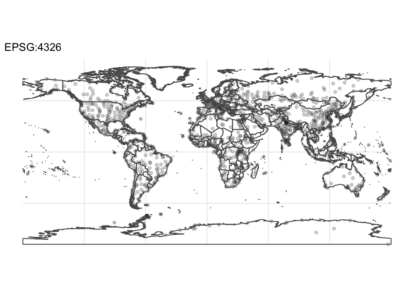
Coordinate reference systems

You can get a coordinate reference system with sf::st_crs. This returns a crs object which has the crs for the user input object as a character string and the well-known text (wkt) for the coordinate reference system.

usa_crs <- st_crs(usa)

usa_crs

Coordinate Reference System:
  User input: WGS 84 
  wkt:
GEOGCRS["WGS 84",
    ENSEMBLE["World Geodetic System 1984 ensemble",
        MEMBER["World Geodetic System 1984 (Transit)"],
        MEMBER["World Geodetic System 1984 (G730)"],
        MEMBER["World Geodetic System 1984 (G873)"],
        MEMBER["World Geodetic System 1984 (G1150)"],
        MEMBER["World Geodetic System 1984 (G1674)"],
        MEMBER["World Geodetic System 1984 (G1762)"],
        MEMBER["World Geodetic System 1984 (G2139)"],
        ELLIPSOID["WGS 84",6378137,298.257223563,
            LENGTHUNIT["metre",1]],
        ENSEMBLEACCURACY[2.0]],
    PRIMEM["Greenwich",0,
        ANGLEUNIT["degree",0.0174532925199433]],
    CS[ellipsoidal,2],
        AXIS["geodetic latitude (Lat)",north,
            ORDER[1],
            ANGLEUNIT["degree",0.0174532925199433]],
        AXIS["geodetic longitude (Lon)",east,
            ORDER[2],
            ANGLEUNIT["degree",0.0174532925199433]],
    USAGE[
        SCOPE["Horizontal component of 3D system."],
        AREA["World."],
        BBOX[-90,-180,90,180]],
    ID["EPSG",4326]]

A crs object also has a method for returning the spatial reference identifier (or SRID). The SRID is a unique identifier for a specific coordinate system, tolerance, and resolution.

Find coordinate reference systems

You can explore a database of over 6000 coordinate reference system with the corresponding EPSG and ESRI SRID codes at EPSG.io. You can also use the crsuggest package which uses data from the EPSG Registry (a product of the International Association of Oil & Gas Producers). The Web Mercator projection or “EPSG:3857” is convenient option that works well for many use cases.

st_crs(usa)$srid

[1] "EPSG:4326"

You can change the coordinate reference system using the sf::st_transform function:

usa_3857 <- st_transform(usa, 3857)

st_crs(usa_3857)

Coordinate Reference System:
  User input: EPSG:3857 
  wkt:
PROJCRS["WGS 84 / Pseudo-Mercator",
    BASEGEOGCRS["WGS 84",
        ENSEMBLE["World Geodetic System 1984 ensemble",
            MEMBER["World Geodetic System 1984 (Transit)"],
            MEMBER["World Geodetic System 1984 (G730)"],
            MEMBER["World Geodetic System 1984 (G873)"],
            MEMBER["World Geodetic System 1984 (G1150)"],
            MEMBER["World Geodetic System 1984 (G1674)"],
            MEMBER["World Geodetic System 1984 (G1762)"],
            MEMBER["World Geodetic System 1984 (G2139)"],
            ELLIPSOID["WGS 84",6378137,298.257223563,
                LENGTHUNIT["metre",1]],
            ENSEMBLEACCURACY[2.0]],
        PRIMEM["Greenwich",0,
            ANGLEUNIT["degree",0.0174532925199433]],
        ID["EPSG",4326]],
    CONVERSION["Popular Visualisation Pseudo-Mercator",
        METHOD["Popular Visualisation Pseudo Mercator",
            ID["EPSG",1024]],
        PARAMETER["Latitude of natural origin",0,
            ANGLEUNIT["degree",0.0174532925199433],
            ID["EPSG",8801]],
        PARAMETER["Longitude of natural origin",0,
            ANGLEUNIT["degree",0.0174532925199433],
            ID["EPSG",8802]],
        PARAMETER["False easting",0,
            LENGTHUNIT["metre",1],
            ID["EPSG",8806]],
        PARAMETER["False northing",0,
            LENGTHUNIT["metre",1],
            ID["EPSG",8807]]],
    CS[Cartesian,2],
        AXIS["easting (X)",east,
            ORDER[1],
            LENGTHUNIT["metre",1]],
        AXIS["northing (Y)",north,
            ORDER[2],
            LENGTHUNIT["metre",1]],
    USAGE[
        SCOPE["Web mapping and visualisation."],
        AREA["World between 85.06°S and 85.06°N."],
        BBOX[-85.06,-180,85.06,180]],
    ID["EPSG",3857]]

You can also check if a object is using a geographic (also known as geodetic or simply lon/lat) or projected coordinate reference system using the sf::st_is_longlat function:

st_is_longlat(usa)

[1] TRUE

st_is_longlat(usa_3857)

[1] FALSE

Tip

Review the sf vignette Spherical geometry in sf using s2geometry for a technical explanation of how sf uses the S2 Geometry Library when manipulating data with a geographic coordinate reference system.

Both ggplot2 and tmap can convert the crs of input objects before mapping. For example, tm_shape supports an optional “projection” argument such as “EPSG:3035” (the Lambert azimuthal equal-area projection):

tm_shape(countries, projection = "EPSG:3035") +
  tm_polygons("grey85", border.col = "grey30") +
  tm_layout(earth.boundary = TRUE, frame = FALSE)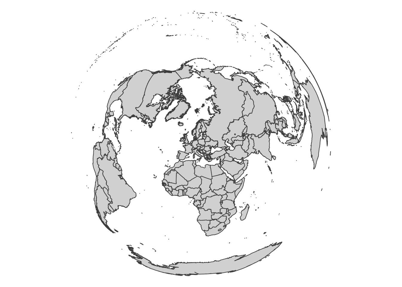

The ggplot2::geom_sf function uses the coordinate reference system of the first sf object provided and re-projects additional objects to match.

library(ggplot2)

countries_3857 <- st_transform(countries, 3857)

ggplot() +
  geom_sf(data = populated_places, alpha = 0.2) +
  geom_sf(data = countries_3857, fill = NA) +
  labs(title = st_crs(populated_places)$srid) +
  theme_minimal()