Get areas and data to layer on a map • mapbaltimore

library(mapbaltimore)
library(getdata)
library(ggplot2)

set_map_theme()

Using the mapbaltimore package starts with understanding the get_baltimore_area() function and getdata function that powers most data access functions in the package: get_location_data().

To show how these different functions work, I’ll make a simple map_area function we will use in this article.

map_area <- function(x, col) {
  ggplot(data = x) +
    geom_sf(aes(fill = .data[[col]])) +
    geom_sf_label(aes(label = .data[[col]])) +
    guides(fill = "none")
}

Get areas

The get_area function uses the dplyr::filter() to select one or more areas of a specified type of political or administrative geography. You can select any one of the seven different types:

Neighborhoods
Baltimore City Council districts
Maryland state legislative districts
U.S. Congressional districts that include Baltimore City
Baltimore City Planning Districts
Baltimore City Police Districts
Baltimore City Community Statistical Areas

Get areas by name or id

You can review the names (name) or identifiers (id) for each type of area by looking at the corresponding column in the data. Typically, the name column should also work as a label for an area and the id column is used as a unique identifier. The names require an exact match. For example, get_baltimore_area(type = "neighborhood", name = "Washington Village/Pigtown") works but get_baltimore_area(type = "neighborhood", name = "Pigtown") will return an error.

# Show the first 3 council district names
council_districts$name[1:3]
#> [1] "District 8" "District 7" "District 6"

# Get district 8 by name
get_baltimore_area(
  type = "council district",
  name = "District 8"
) %>%
  map_area("name")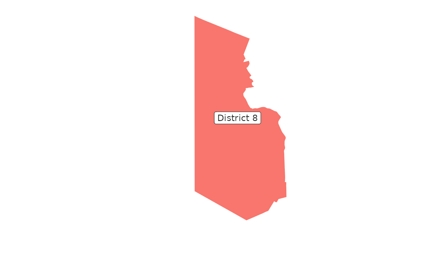


# Show the first 3 council district ids
council_districts$id[1:3]
#> [1] "8" "7" "6"

# Get district 7 by id
get_baltimore_area(
  type = "council district",
  id = 7
) %>%
  map_area("id")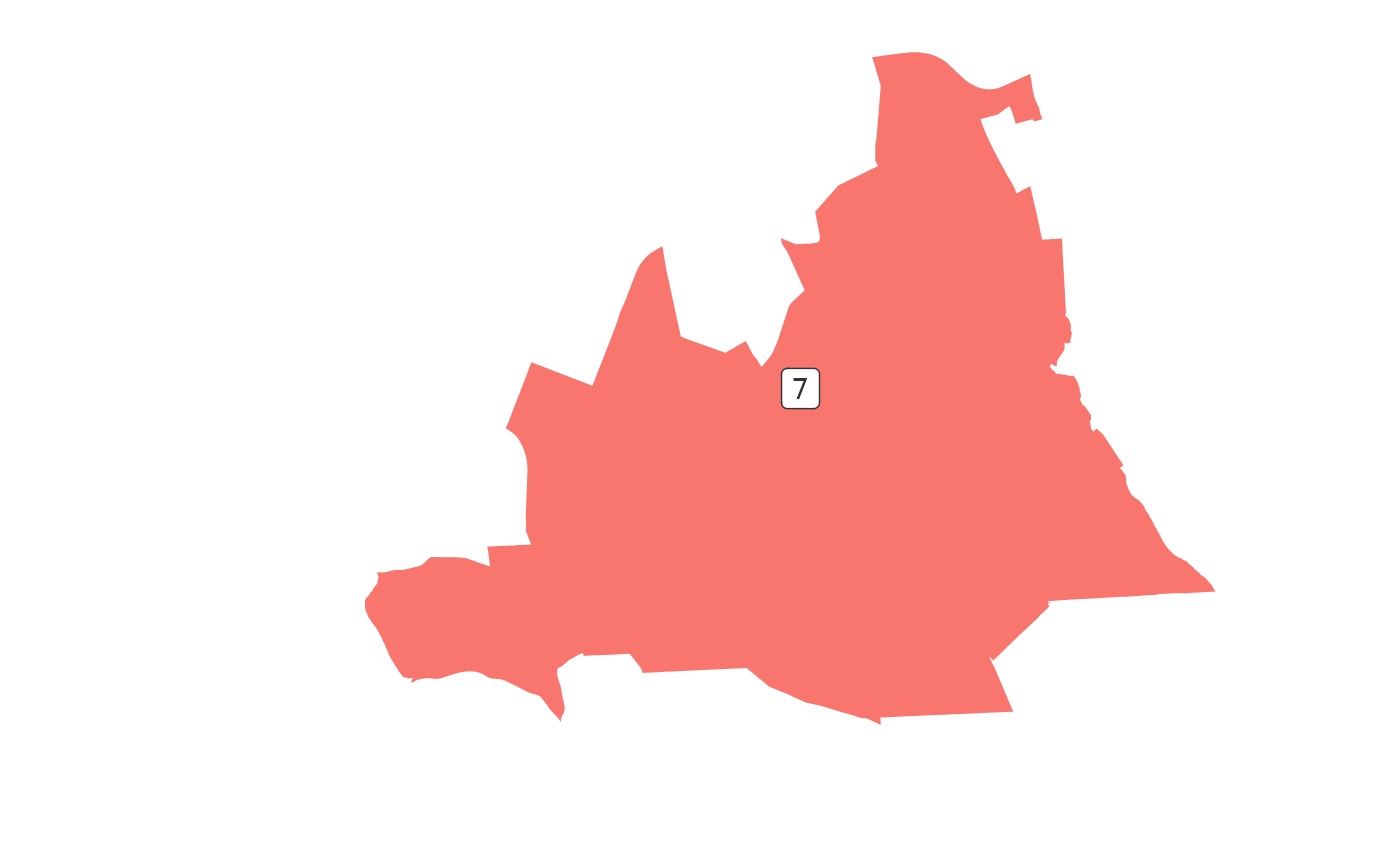

Get multiple areas

To return multiple areas, you can provide a vector of names or identifiers.

area_multiple <- get_baltimore_area(
  type = "neighborhood",
  name = c("Mount Vernon", "Mid-Town Belvedere", "Seton Hill")
)

area_multiple %>%
  map_area("name")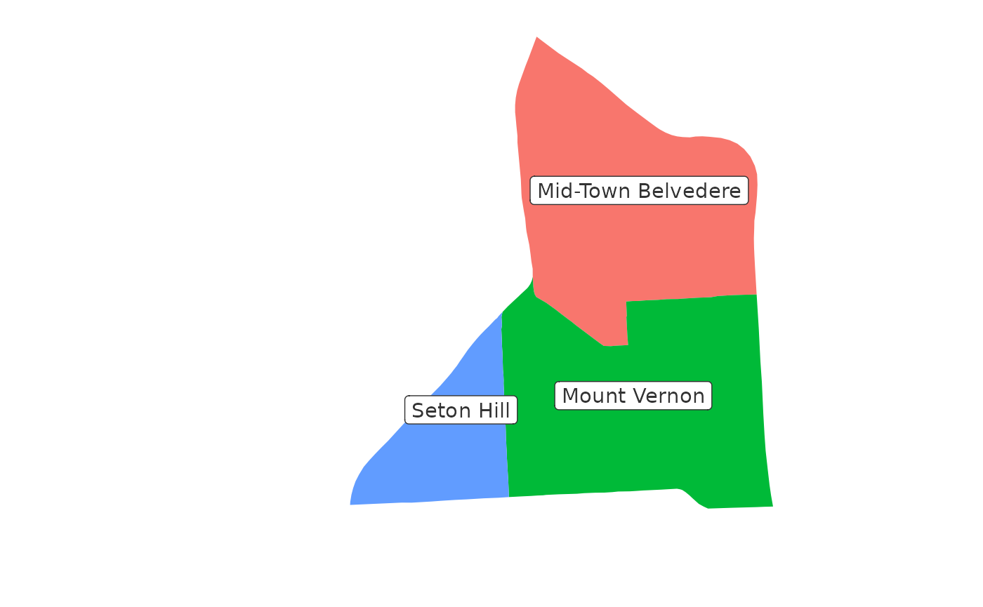

You can also combine multiple areas into a single simple feature using the union parameter. This is helpful when you want to get data for multiple neighborhoods at the same time or map them as a single combined area.

By default the area names are concatenated using a ampersand separator, however, the length of these combined names are difficult to fit on a map and it is often better to replace the name with a shorter alternative.

area_multiple_union <- get_baltimore_area(
  type = "neighborhood",
  name = c("Mount Vernon", "Mid-Town Belvedere", "Seton Hill"),
  union = TRUE
)

area_multiple_union$name
#> [1] "Mid-Town Belvedere, Mount Vernon, and Seton Hill"

area_multiple_union$name <- "Mount Vernon area"

area_multiple_union %>%
  map_area("name")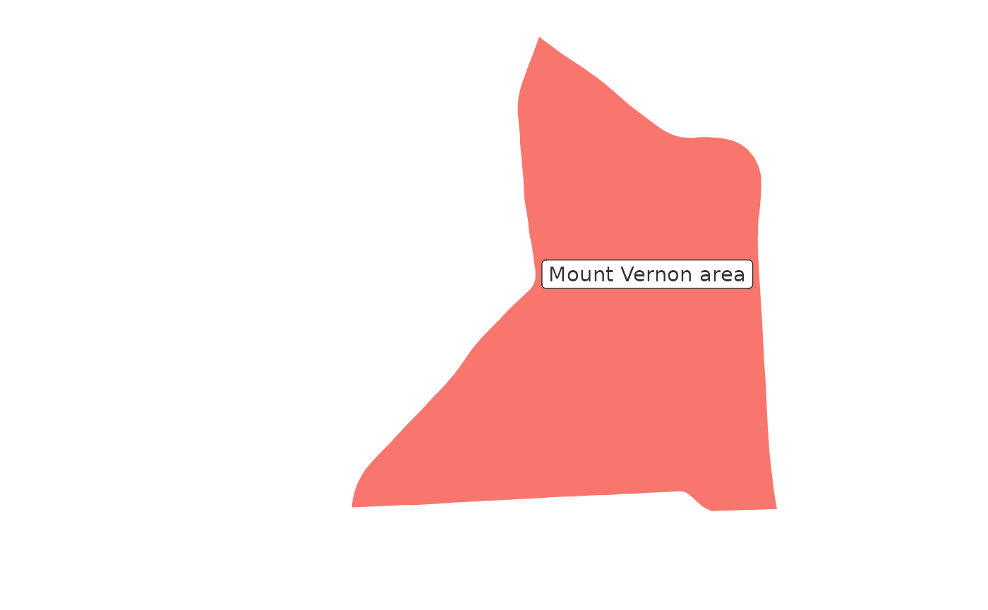

Get data for an area

The get_area_data() function offers a great deal of flexibility. You can provide an area from get_area() or any other simple feature polygon or multipolygon located within Baltimore City (or any region if using cached baltimore_msa_streets data set). You can also provide a bounding box created with the sf::st_bbox() function.

To illustrate the options for this function, I’m getting the downtown neighborhood as a simple feature object (area) and making a list with ggplot2 layers, guide, and scale (area_layer) that I reuse below for the example maps in this section.

area <- get_baltimore_area(
  type = "neighborhood",
  name = "Downtown"
)

area_layer <- list(
  geom_sf(data = area, fill = "grey90", alpha = 0.8, color = "grey20", linetype = "dotted"),
  geom_sf_label(data = area, aes(label = name)),
  guides(fill = "none"),
  scale_fill_viridis_d()
)

Adjust the area bounding box

In order to place an area in context, you may want a portion of data for the surrounding area so the function returns data within the bounding box of the area by default. The dimensions of this bounding box can be adjusted using the dist, diag_ratio, and asp parameters. You can access these adjustments directly using the buffer_area(), adjust_bbox_asp(), and adjust_bbox() functions. These functions are used below to illustrate how they work when you use the corresponding parameters with get_area_data().

The dist parameter is passed to the sf::st_buffer() function and is used to set the buffer in meters for the area. The diag_ratio is also used to set a buffer distances but the number represents the proportion of the diagonal distance of the area bounding box. This is helpful because a set ratio will scale in proportion to the size of the area.

example_dist <- 50
example_diag_ratio <- 0.25

# 50 meter buffer
area_dist <- sfext::st_buffer_ext(area, dist = example_dist)
area_dist_bbox <- sfext::sf_bbox_to_sf(sf::st_bbox(area_dist))

# buffer 1/4 (0.25) of the diagonal distance of the bounding box
area_diag_ratio <- sfext::st_buffer_ext(area, diag_ratio = example_diag_ratio)
area_diag_ratio_bbox <- sfext::sf_bbox_to_sf(sf::st_bbox(area_diag_ratio))

ggplot() +
  geom_sf(data = area_dist, fill = "purple", alpha = 0.1) +
  geom_sf(data = area_dist_bbox, color = "purple", fill = NA) +
  geom_sf(data = area_diag_ratio, fill = "darkorange", alpha = 0.1) +
  geom_sf(data = area_diag_ratio_bbox, color = "darkorange", fill = NA) +
  area_layer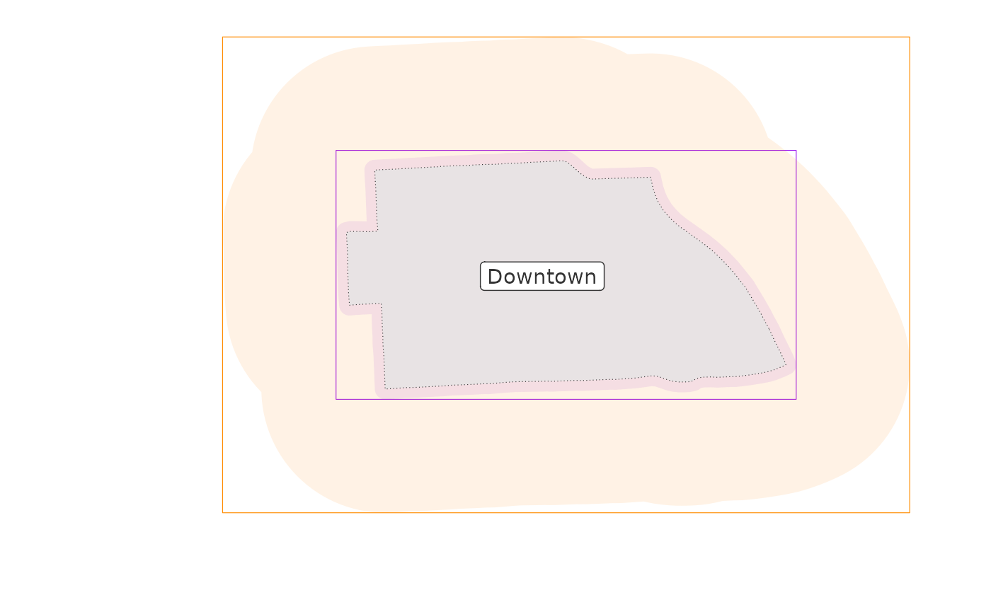

The asp parameter is applied after any buffers are applied. The adjust_bbox_asp() function accepts either a number, e.g. 1.5, or a string in the format most commonly used for aspect ratios, e.g. “6:4”. This example shows the extent of a square bounding box for both the buffered downtown areas created above.

example_asp <- "1:1"

area_dist_asp <- sfext::st_bbox_asp(area_dist, asp = example_asp) %>%
  sfext::sf_bbox_to_sf()

area_diag_ratio_asp <- sfext::st_bbox_asp(area_diag_ratio, asp = example_asp) %>%
  sfext::sf_bbox_to_sf()

ggplot() +
  geom_sf(data = area_dist_asp, fill = "purple", color = "purple", alpha = 0.1) +
  geom_sf(data = area_diag_ratio_asp, fill = "darkorange", color = "darkorange", alpha = 0.1) +
  area_layer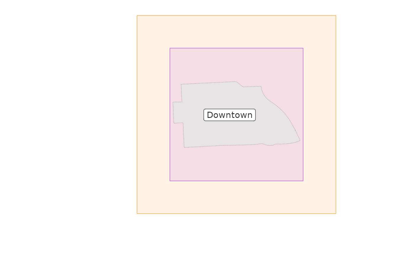

Cropping and trimming data

Finally, here is how these area adjustments work in combination with the get_location_data() function. By default, the data is cropped to the bounding box of the provided area:

get_location_data(
  location = area,
  data = council_districts
) %>%
  map_area("name") +
  area_layer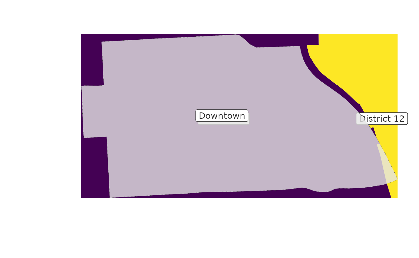

Here is the data with a diag_ratio buffer:

get_location_data(
  location = area,
  data = council_districts,
  diag_ratio = example_diag_ratio
) %>%
  map_area("name") +
  area_layer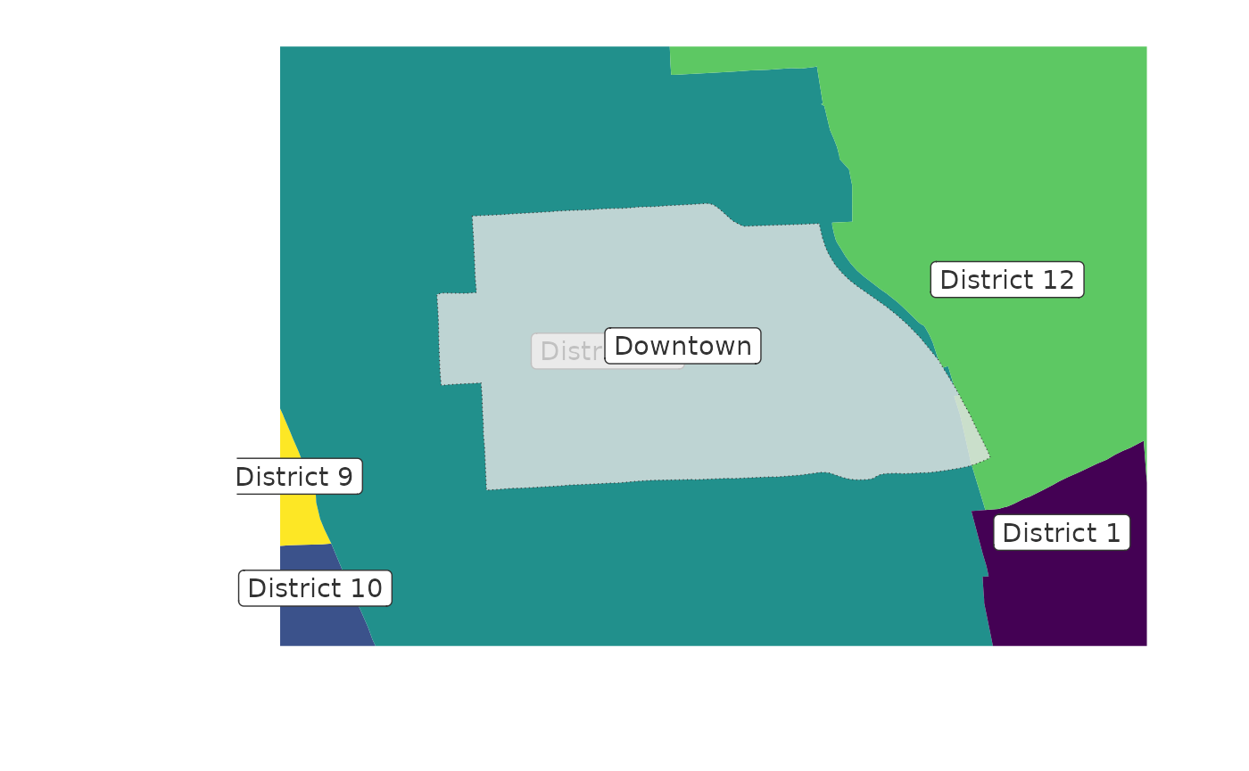

Here is the data using an asp adjustment to return a square :

get_location_data(
  location = area,
  data = council_districts,
  asp = example_asp
) %>%
  map_area("name") +
  area_layer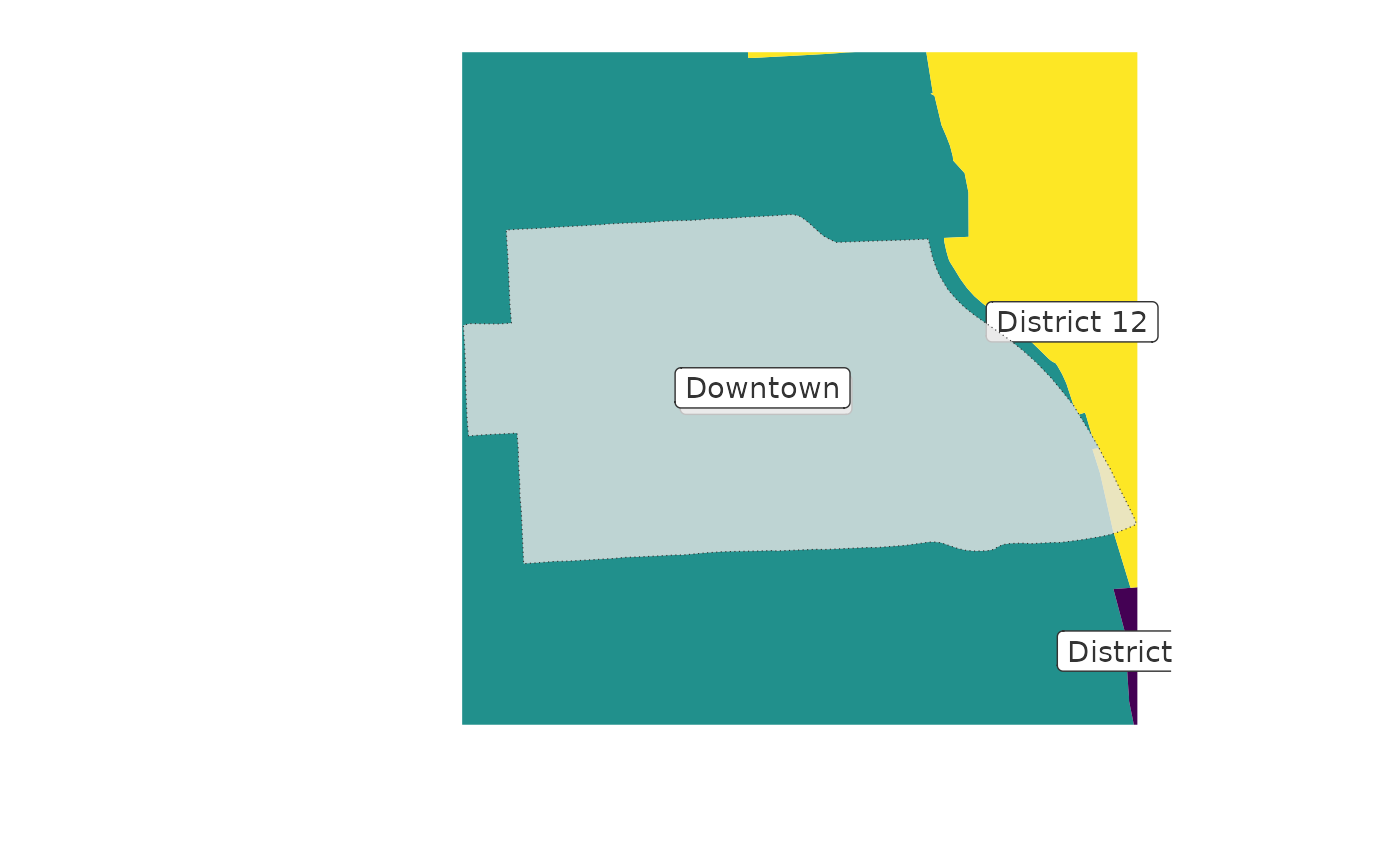

You can also avoid cropping if you want to return the full extent of any data that even partially overlaps with the area or bounding box. For example, this is the same example as above with crop = FALSE.

get_location_data(
  location = area,
  data = council_districts,
  crop = FALSE
) %>%
  map_area("name") +
  area_layer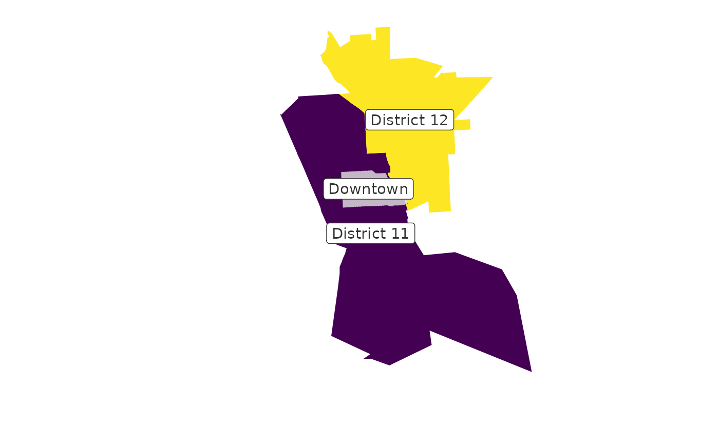

If you want to use crop = FALSE in combination with the area adjustment parameters you must either supply a bounding box instead of an area or adjust the area using buffer_area() before passing it to the get_area_data() function. The maps are similar enough to the prior example that I’ve hid the results but provided the code here as a sample.

get_location_data(
  location = sfext::st_buffer_ext(area, diag_ratio = example_diag_ratio),
  data = council_districts,
  crop = FALSE
)

get_location_data(
  location = sf::st_bbox(area),
  data = council_districts,
  diag_ratio = example_diag_ratio,
  crop = FALSE
)

Depending on the type of data you are working with, you may also want to trim the data to the area using the sf::st_intersection() function. You can’t trim to an area if you only provide a bounding box (bbox); you must provide an area.

area_trees <- get_location_data(
  location = sf::st_bbox(area),
  data = "trees",
  dist = example_dist,
  from_crs = 2804,
  package = "mapbaltimore"
)

area_trees_trimmed <- get_location_data(
  location = area,
  data = "trees",
  dist = example_dist,
  trim = TRUE,
  package = "mapbaltimore"
)

ggplot() +
  area_layer +
  geom_sf(data = area_trees, color = "wheat3") +
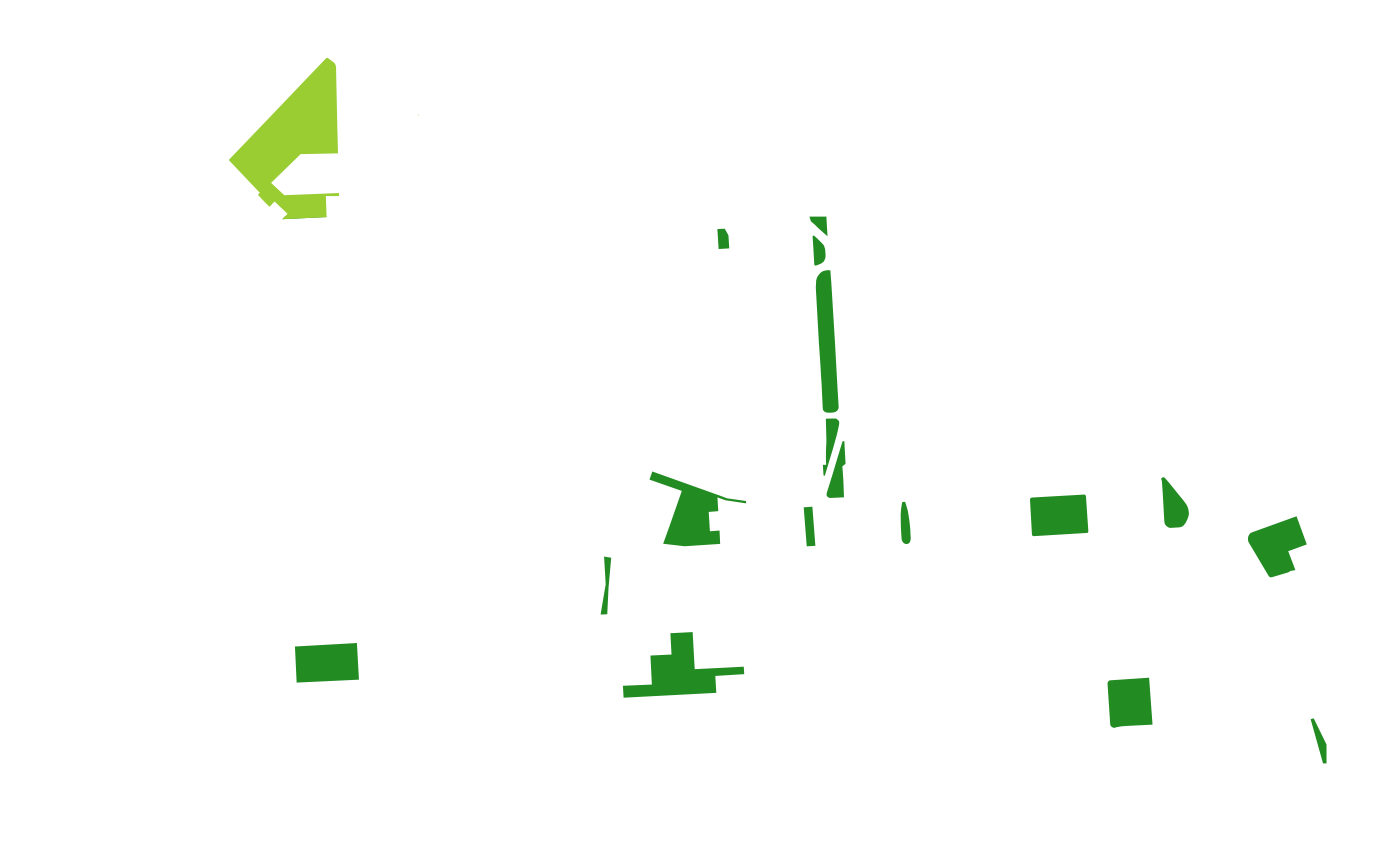
  geom_sf(data = area_trees_trimmed, color = "forestgreen", alpha = 0.8)

Similar to crop, using the trim = TRUE parameter ignores any distance adjustments but the same work around can be used to apply a buffer to the area before passing it to get_area_data().

area_trees_trimmed_diag_ratio <- get_location_data(
  location = sfext::st_buffer_ext(area, diag_ratio = example_diag_ratio),
  data = "trees",
  pkg = "mapbaltimore",
  trim = TRUE
)

ggplot() +
  area_layer +
  geom_sf(data = area_trees_trimmed_diag_ratio, color = "forestgreen") +
  geom_sf(data = area_trees_trimmed, color = "wheat3")

The trim parameter is also supported by the get_location_data() and get_osm_data() functions that are discussed in more detail in the article on external, cached, and remote data sources.

Layering data in area maps

You may be wondering why these all of these parameters may be useful. The maplayer::layer_location_data() function combines get_location_data() with ggplot2::geom_sf() to quickly turn the data from mapbaltimore into ggplot maps. Here is a simple example that turns streets and parks data into a map of the downtown area.

example_diag_ratio <- 0.05

layer_streets <- maplayer::layer_location_data(
  location = area,
  data = streets,
  color = "gray60",
  diag_ratio = example_diag_ratio
)

layer_parks <- maplayer::layer_location_data(
  location = area,
  data = parks,
  fill = "forestgreen",
  diag_ratio = example_diag_ratio
)

background_layers <- list(layer_streets, layer_parks)

ggplot() +
  background_layers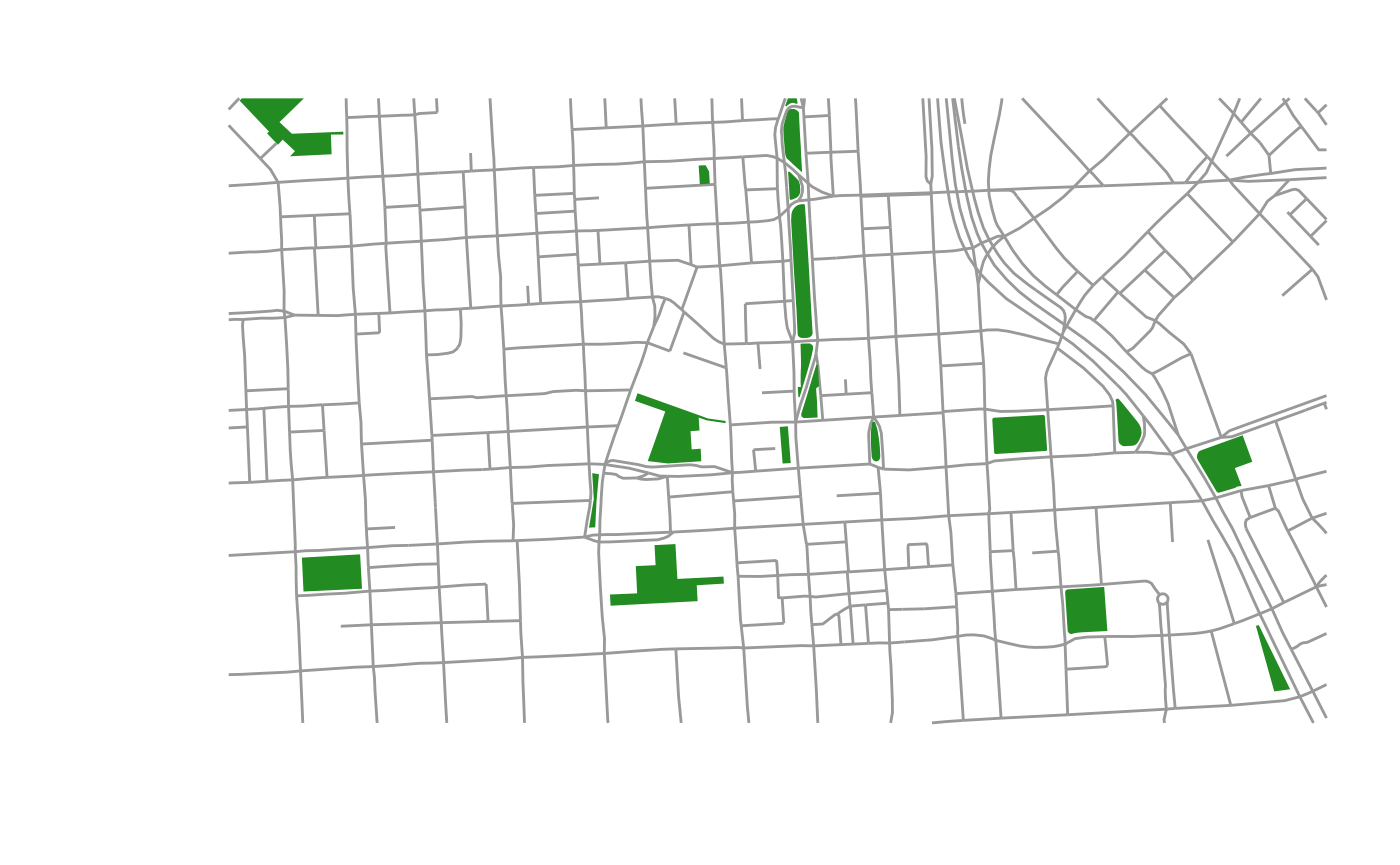

The following example shows how to create a new map layer using data imported from Open Street Map. When no location is provided, no filtering takes place.

layer_area_buildings <- maplayer::layer_location_data(
  data = getdata::get_osm_data(
    location = area,
    diag_ratio = example_diag_ratio,
    key = "building",
    value = "yes",
    geometry = "polygons"
  ),
  fill = "antiquewhite2",
  color = NA,
  alpha = 1
)
#> ℹ OpenStreetMap data is licensed under the Open Database License (ODbL).
#>   Attribution is required if you use this data.
#> • Learn more about the ODbL and OSM attribution requirements at
#>   <https://www.openstreetmap.org/copyright>
#> This message is displayed once every 8 hours.

ggplot() +
  background_layers +
  layer_area_buildings +
  labs(caption = "© OpenStreetMap contributors")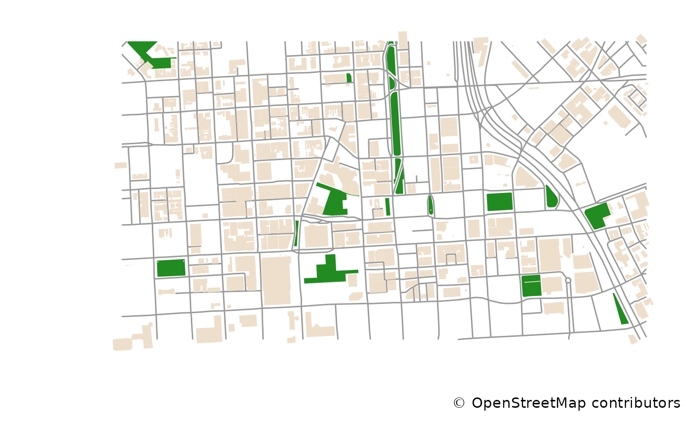

You can also pass a url to add data from any ArcGIS MapServer or FeatureServer.

parking_facility_url <- "https://opendata.baltimorecity.gov/egis/rest/services/Hosted/Parking_Facilities/FeatureServer/0"

layer_area_parking <- maplayer::layer_location_data(
  location = area,
  data = parking_facility_url,
  diag_ratio = example_diag_ratio,
  color = "gray10",
  fill = "yellow",
  shape = 24,
  size = 4
)

ggplot() +
  background_layers +
  layer_area_buildings +
  layer_area_parking +
  ggtitle("Parking facilities in Downtown Baltimore")

Finally, you can apply some additional function to the data using the same lambda syntax used for purrr. For example, the tree data includes dead trees which could be removed before displaying them on a map.

layer_area_trees <- list(
  maplayer::layer_location_data(
    location = area,
    data = "trees.gpkg",
    package = "mapbaltimore",
    fn = ~ dplyr::filter(.x, condition != "Dead"),
    trim = TRUE,
    mapping = aes(
      size = dbh * 0.4,
      color = factor(condition, c("Good", "Fair", "Poor"))
    ),
    alpha = 0.6
  ),
  guides(size = "none"),
  labs(color = "Tree condition"),
  scale_color_manual(values = shades::gradient(c("forestgreen", "burlywood4"), 3))
)

ggplot() +
  background_layers +
  layer_area_trees

Working with multiple areas

There are a few different ways to use these functions with a dataframe of multiple areas. The get_area_data() function always combines multiple areas into a single geometry and returns data for a bounding box that encompasses all areas.

If you want to get data for each area separately, the dplyr::nest_by() and purrr::map_dfr() functions can be used. The following example also shows how get_nearby_areas() can be used to return a data frame of overlapping or immediately surrounding areas.

nearby_areas <- get_nearby_areas(area = area, type = "neighborhood")

nearby_areas_nested <- dplyr::nest_by(nearby_areas, name, .keep = TRUE)

nearby_parks <- purrr::map_dfr(
  nearby_areas_nested$data,
  ~ getdata::get_location_data(
    location = .x,
    data = parks,
    trim = TRUE
  ) %>%
    dplyr::bind_cols(neighborhood = .x$name)
)

# FIXME: This isn't working!
# ggplot() +
#   maplayer::layer_location_data(location = nearby_areas, data = streets, trim = TRUE, color = "gray70", crs = 2804) +
#  # layer_parks +
#  ggplot2::geom_sf(data = sf::st_make_valid(nearby_parks), aes(fill = neighborhood)) +
#  # scale_fill_viridis_d() +
#   labs(fill = "Neighborhood\nof park")

Another approach relies on using the data inherited from ggplot() with the option to apply different aesthetics or process the data differently in each layer of the map.

parks %>%
  ggplot() +
  maplayer::layer_location_data(location = area, trim = TRUE, fill = "forestgreen") +
  maplayer::layer_location_data(location = nearby_areas[6, ], trim = TRUE, fill = "yellowgreen")