Introduction to sfext • sfext

library(sfext)
library(dplyr)
library(ggplot2)

theme_set(theme_void())

The {sfext} package has several categories of functions:

Functions for reading and writing spatial data
Converting the class or geometry of objects
Modifying sf, sfc, and bbox objects
Getting information about sf, sfc, and bbox objects
Working with units and scales

Reading and writing sf objects

Reading sf objects

read_sf_ext() calls one of four other functions depending on the input parameters:

read_sf_path() is similar to sf::read_sf but has a few additional features. It checks the existence of a file before reading, supports the creation of wkt_filter parameters based on a bounding box, and supports conversion of tabular data to simple feature objects.

nc <- read_sf_ext(path = system.file("shape/nc.shp", package = "sf"))
# This is equivalent to read_sf_path(system.file("shape/nc.shp", package = "sf"))
# Or sf::read_sf(dsn = system.file("shape/nc.shp", package = "sf"))

glimpse(nc)
#> Rows: 100
#> Columns: 15
#> $ AREA      <dbl> 0.114, 0.061, 0.143, 0.070, 0.153, 0.097, 0.062, 0.091, 0.11…
#> $ PERIMETER <dbl> 1.442, 1.231, 1.630, 2.968, 2.206, 1.670, 1.547, 1.284, 1.42…
#> $ CNTY_     <dbl> 1825, 1827, 1828, 1831, 1832, 1833, 1834, 1835, 1836, 1837, …
#> $ CNTY_ID   <dbl> 1825, 1827, 1828, 1831, 1832, 1833, 1834, 1835, 1836, 1837, …
#> $ NAME      <chr> "Ashe", "Alleghany", "Surry", "Currituck", "Northampton", "H…
#> $ FIPS      <chr> "37009", "37005", "37171", "37053", "37131", "37091", "37029…
#> $ FIPSNO    <dbl> 37009, 37005, 37171, 37053, 37131, 37091, 37029, 37073, 3718…
#> $ CRESS_ID  <int> 5, 3, 86, 27, 66, 46, 15, 37, 93, 85, 17, 79, 39, 73, 91, 42…
#> $ BIR74     <dbl> 1091, 487, 3188, 508, 1421, 1452, 286, 420, 968, 1612, 1035,…
#> $ SID74     <dbl> 1, 0, 5, 1, 9, 7, 0, 0, 4, 1, 2, 16, 4, 4, 4, 18, 3, 4, 1, 1…
#> $ NWBIR74   <dbl> 10, 10, 208, 123, 1066, 954, 115, 254, 748, 160, 550, 1243, …
#> $ BIR79     <dbl> 1364, 542, 3616, 830, 1606, 1838, 350, 594, 1190, 2038, 1253…
#> $ SID79     <dbl> 0, 3, 6, 2, 3, 5, 2, 2, 2, 5, 2, 5, 4, 4, 6, 17, 4, 7, 1, 0,…
#> $ NWBIR79   <dbl> 19, 12, 260, 145, 1197, 1237, 139, 371, 844, 176, 597, 1369,…
#> $ geometry  <MULTIPOLYGON [°]> MULTIPOLYGON (((-81.47276 3..., MULTIPOLYGON ((…

bbox <- as_bbox(nc[10, ])

nc_in_bbox <- read_sf_ext(path = system.file("shape/nc.shp", package = "sf"), bbox = bbox)

nc_basemap <-
  ggplot() +
  geom_sf(data = nc)

nc_basemap +
  geom_sf(data = nc_in_bbox, fill = "red")

The second, read_sf_url(), that supports reading url that are already supported by sf::read_sf but also supports ArcGIS Feature Layers (using the {esri2sf} package) and URLs for tabular data (including both CSV files and Google Sheets). Several functions also support queries based on a name and name_col value (generating a simple SQL query) based on the provided values.

sample_esri_url <- "https://services.arcgis.com/P3ePLMYs2RVChkJx/ArcGIS/rest/services/USA_Boundaries_2022/FeatureServer/1"
states <- read_sf_esri(url = sample_esri_url)
#> ── Downloading "USA_State" from <https://services.arcgis.com/P3ePLMYs2RVChkJx/Ar
#> Layer type: "Feature Layer"
#> Geometry type: "esriGeometryPolygon"
#> Service CRS: "EPSG:4326"
#> Output CRS: "EPSG:4326"
#> 
# This is equivalent to read_sf_url(sample_esri_url)
# Or esri2sf::esri2sf(url = sample_esri_url)

# read_sf_esri and read_sf_query both support the name and name_col parameters
# These parameters also work with read_sf_pkg for cached and extdata files
nc_esri <- read_sf_ext(url = sample_esri_url, name_col = "STATE_NAME", name = "North Carolina")
#> ── Downloading "USA_State" from <https://services.arcgis.com/P3ePLMYs2RVChkJx/Ar
#> Layer type: "Feature Layer"
#> Geometry type: "esriGeometryPolygon"
#> Service CRS: "EPSG:4326"
#> Output CRS: "EPSG:4326"
#> 

ggplot() +
  geom_sf(data = states) +
  geom_sf(data = nc_esri, fill = "red")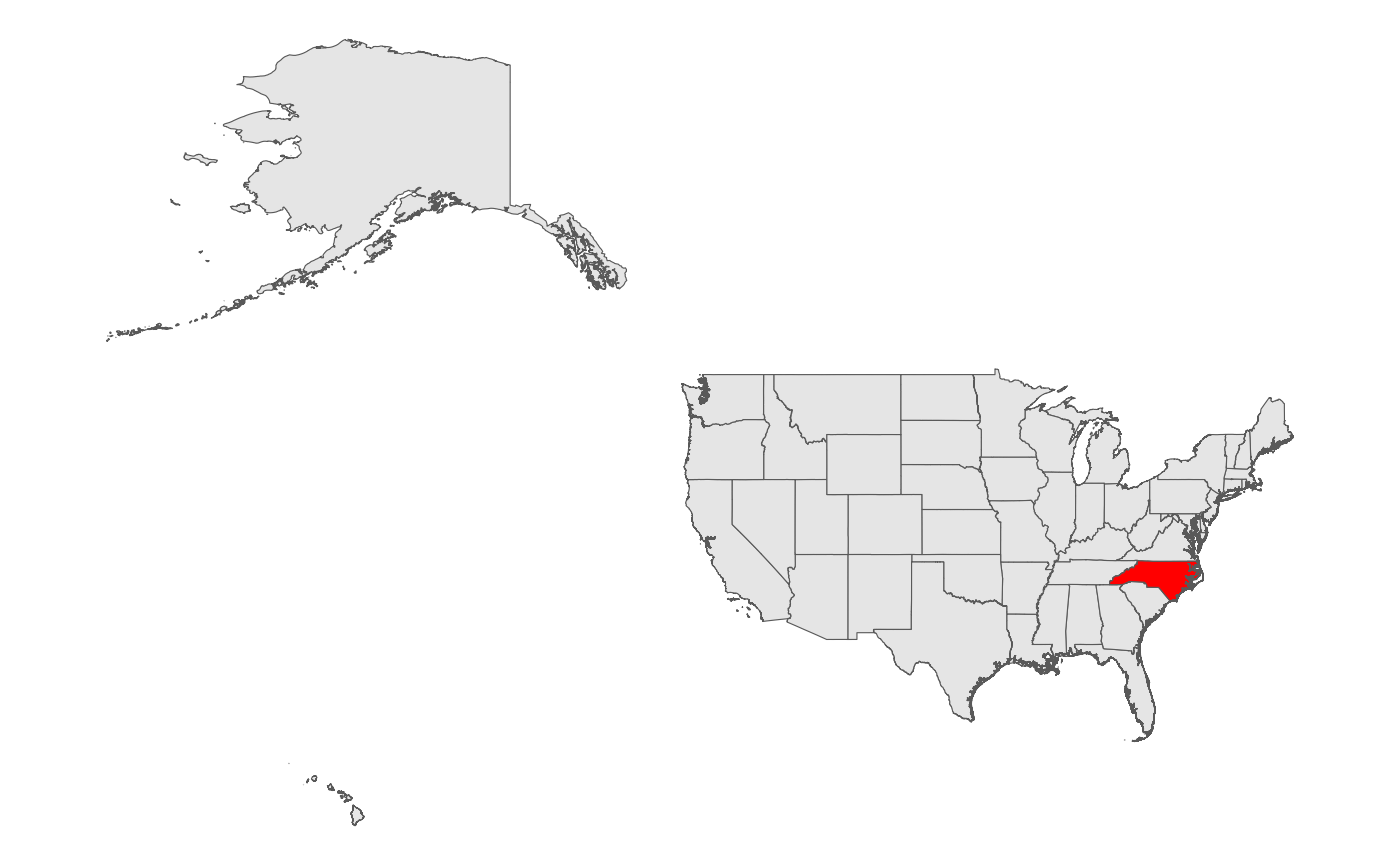

The read functions also support URLs for GitHub Gists (assuming the first file in the Gist is a spatial data file) or Google MyMaps.

gmap_data <- read_sf_ext(url = "https://www.google.com/maps/d/u/0/viewer?mid=1CEssu_neU7lx_vAZs5qpufOBoUQ&ll=-3.81666561775622e-14%2C0&z=1")

ggplot() +
  geom_sf(data = gmap_data[2, ])

The third, read_sf_pkg(), can load spatial data from any installed package including exported data, files in the extdata folder, or data in a package-specific cache folder. This is particularly useful when working with spatial data packages such as {mapbaltimore} or {mapmaryland}.

The fourth, read_sf_query(), is most similar to sf::read_sf but provides an optional spatial filter based on the bbox parameter and supports the creation of queries using a basic name and name_col parameter.

Writing sf objects

write_sf_ext() wraps sf::write_sf but uses filenamr::make_filename() to support the creation of consistent file names using labels or date prefixes to organize exports.

filenamr::make_filename(
  name = "Ashe County",
  label = "NC",
  prefix = "date",
  fileext = "gpkg"
)
#> [1] "2024-01-12_nc_ashe_county.gpkg"

write_sf_ext() also supports the automatic creation of destination folders and the use of a package-specific cache folder created by rappdirs::user_cache_dir(). These functions are now in the filenamr package.

Converting sf objects

Checking and converting sf objects

There are several helper functions that are used extensively by the package itself. While these conversions are easy to do with existing {sf} functions, these alternatives follow a tidyverse style syntax and support a wider range of input values.

is_sf(nc)
#> [1] TRUE

is_sfc(nc$geometry)
#> [1] TRUE

nc_bbox <- as_bbox(nc)

is_bbox(nc_bbox)
#> [1] TRUE

The ext parameter can be used to make is_sf() more general allowing sf, sfc, or bbox objects instead of just sf objects.

is_sf(nc$geometry)
#> [1] FALSE

is_sf(nc$geometry, ext = TRUE)
#> [1] TRUE

There are similar functions for checking and converting the geometry type for an object including is_point(), is_polygon(), is_line(), and others.

is_point(nc)
#> [1] FALSE

is_point(suppressWarnings(sf::st_centroid(nc)))
#> [1] TRUE

# as_point returns an sfg object
is_sfg(as_point(nc))
#> [1] TRUE

# as_points returns an sfc object (and accepts numeric inputs as well as sfg)
is_sfc(as_points(c(-79.40065, 35.55937), crs = 4326))
#> [1] TRUE

Converting to and from data frames

By default the conversion from sf to data frame object, uses the centroid of any polygon. It can also use a surface point from sf::st_point_on_surface

df_centroid <- sf_to_df(nc_in_bbox)
df_surface_point <- sf_to_df(nc_in_bbox, geometry = "surface point")

These can be converted back to an sf object but the point geometry is used instead of the original polygon:

df_centroid_sf <- df_to_sf(df_centroid, crs = 3857)
df_surface_point_sf <- df_to_sf(df_surface_point, crs = 3857)

df_example_map <-
  ggplot() +
  geom_sf(data = nc_in_bbox) +
  geom_sf(data = df_centroid_sf, color = "red", size = 3) +
  geom_sf(data = df_surface_point_sf, color = "blue", size = 2)

df_example_map

Alternatively, sf_to_df() can also use well known text as an output format:

df_wkt <- sf_to_df(nc_in_bbox, geometry = "wkt")

glimpse(df_wkt)
#> Rows: 5
#> Columns: 15
#> $ AREA      <dbl> 0.143, 0.124, 0.153, 0.108, 0.170
#> $ PERIMETER <dbl> 1.630, 1.428, 1.616, 1.483, 1.680
#> $ CNTY_     <dbl> 1828, 1837, 1839, 1900, 1903
#> $ CNTY_ID   <dbl> 1828, 1837, 1839, 1900, 1903
#> $ NAME      <chr> "Surry", "Stokes", "Rockingham", "Forsyth", "Guilford"
#> $ FIPS      <chr> "37171", "37169", "37157", "37067", "37081"
#> $ FIPSNO    <dbl> 37171, 37169, 37157, 37067, 37081
#> $ CRESS_ID  <int> 86, 85, 79, 34, 41
#> $ BIR74     <dbl> 3188, 1612, 4449, 11858, 16184
#> $ SID74     <dbl> 5, 1, 16, 10, 23
#> $ NWBIR74   <dbl> 208, 160, 1243, 3919, 5483
#> $ BIR79     <dbl> 3616, 2038, 5386, 15704, 20543
#> $ SID79     <dbl> 6, 5, 5, 18, 38
#> $ NWBIR79   <dbl> 260, 176, 1369, 5031, 7089
#> $ wkt       <chr> "POLYGON ((-80.45612 36.2427, -80.47617 36.25487, -80.53666 …

df_example_map +
  geom_sf(data = df_to_sf(df_wkt), color = "orange", fill = NA)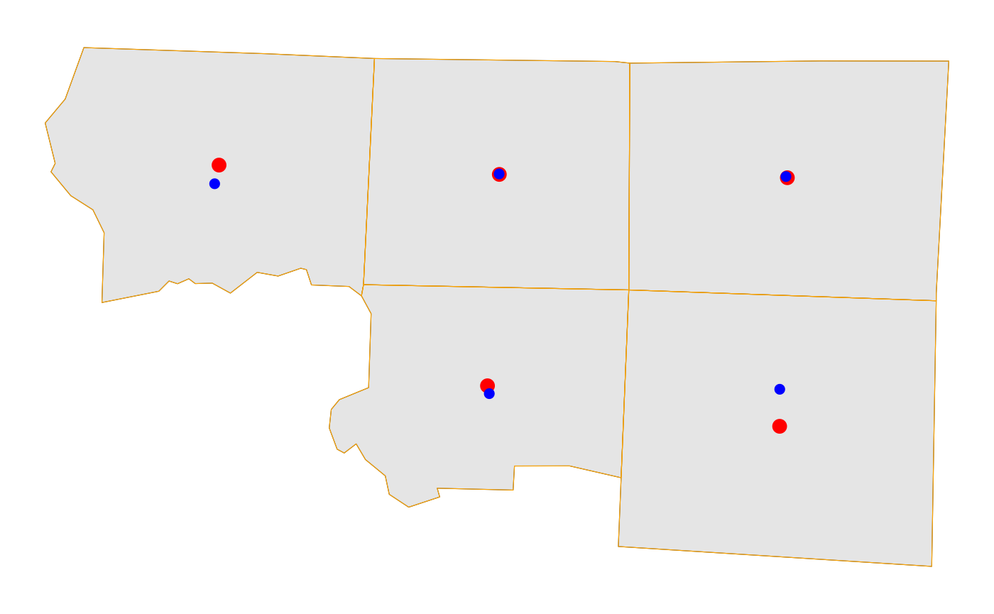

The tidygeocoder package is also used to support conversion of address vectors or data frames.

address_to_sf(x = c("350 Fifth Avenue, New York, NY 10118"))
#> Passing 1 address to the Nominatim single address geocoder
#> Query completed in: 1.7 seconds
#> Simple feature collection with 1 feature and 3 fields
#> Attribute-geometry relationships: constant (3)
#> Geometry type: POINT
#> Dimension:     XY
#> Bounding box:  xmin: -72.366 ymin: 41.10336 xmax: -72.366 ymax: 41.10336
#> Geodetic CRS:  WGS 84
#> # A tibble: 1 × 4
#>   address                                lat   lon           geometry
#> * <chr>                                <dbl> <dbl>        <POINT [°]>
#> 1 350 Fifth Avenue, New York, NY 10118  41.1 -72.4 (-72.366 41.10336)

Modifying sf objects

The next group of functions often provide similar functionality to standard {sf} functions but, again, allow a wider range of inputs and outputs or offer extra features. For example, st_bbox_ext() also wraps sf::st_buffer and uses a helper function based on units::set_units to a buffer distance of any valid distance unit.

nc_bbox <- st_bbox_ext(nc, class = "sf")
# Similar to sf::st_sf(sf::st_as_sfc(sf::st_bbox(nc)))

nc_bbox_buffer <- st_bbox_ext(nc, dist = 50, unit = "mi", class = "sf")
# Similar to sf::st_buffer(nc, dist = units::as_units(50, "mi"))

nc_basemap +
  geom_sf(data = nc_bbox, fill = NA, color = "blue") +
  geom_sf(data = nc_bbox_buffer, fill = NA, color = "red")

Other notable functions in this category include:

st_transform_ext(): takes sf, sfc, or bbox objects as the crs parameter for sf::st_transform() and supports lists of sf objects (look for the allow_list = TRUE parameter to see which functions support lists)
st_union_ext(): unions geometry while also collapsing a name column into a single character string using the cli::pluralize function
st_erase(): checks the validity of inputs with sf::st_is_valid before and after using sf::st_difference or (if flip = TRUE) sf::st_difference

Getting information about sf, sfc, and bbox objects

There are also several functions that return information about the geometry of input objects. Typically, these functions bind the information as a new column to an existing sf input (and convert sfc input objects to sf results).

The get_length() function wraps sf::st_length and (for POLYGON geometries only) lwgeom::st_perimeter:

example_line <- as_line(as_point(nc[1, ]), as_point(nc[2, ]), crs = 4326)

glimpse(get_length(example_line))
#> Rows: 1
#> Columns: 2
#> $ length   [m] 34020.35 [m]
#> $ geometry <LINESTRING [°]> LINESTRING (-81.49823 36.43...

The get_area() function wraps sf::st_area():

glimpse(get_area(nc[1:3, ], unit = "mi^2"))
#> Rows: 3
#> Columns: 16
#> $ AREA      <dbl> 0.114, 0.061, 0.143
#> $ PERIMETER <dbl> 1.442, 1.231, 1.630
#> $ CNTY_     <dbl> 1825, 1827, 1828
#> $ CNTY_ID   <dbl> 1825, 1827, 1828
#> $ NAME      <chr> "Ashe", "Alleghany", "Surry"
#> $ FIPS      <chr> "37009", "37005", "37171"
#> $ FIPSNO    <dbl> 37009, 37005, 37171
#> $ CRESS_ID  <int> 5, 3, 86
#> $ BIR74     <dbl> 1091, 487, 3188
#> $ SID74     <dbl> 1, 0, 5
#> $ NWBIR74   <dbl> 10, 10, 208
#> $ BIR79     <dbl> 1364, 542, 3616
#> $ SID79     <dbl> 0, 3, 6
#> $ NWBIR79   <dbl> 19, 12, 260
#> $ area      [mi^2] 439.0398 [mi^2], 235.8760 [mi^2], 549.4795 [mi^2]
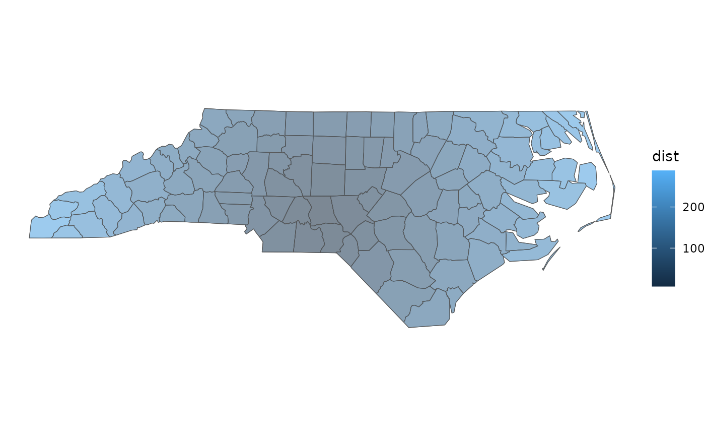
#> $ geometry  <MULTIPOLYGON [°]> MULTIPOLYGON (((-81.47276 3..., MULTIPOLYGON (((-81.23989 3.…

get_dist() supports a more varied range of options including using the “to” parameter to define a corner or center of the input sf object bounding box.

nc <- sf::st_transform(nc, 3857)

# use drop = TRUE, to drop the units class and return a numeric column
dist_example_min <- get_dist(nc, to = c("xmin", "ymin"), unit = "mi", drop = TRUE)

glimpse(select(dist_example_min, NAME, dist))
#> Rows: 100
#> Columns: 3
#> $ NAME     <chr> "Ashe", "Alleghany", "Surry", "Currituck", "Northampton", "He…
#> $ dist     <dbl[,1]> <matrix[26 x 1]>
#> $ geometry <MULTIPOLYGON [m]> MULTIPOLYGON (((-9069486 43..., MULTIPOLYGON (((-9043562 …

nc_basemap +
  geom_sf(data = dist_example_min, aes(fill = dist), alpha = 0.5)


dist_example_mid <- get_dist(nc, to = c("xmid", "ymid"), unit = "mi", drop = TRUE)

nc_basemap +
  geom_sf(data = dist_example_mid, aes(fill = dist), alpha = 0.5)