Working with simple feature and bounding box objects

library(overedge)
library(mapbaltimore)
#> 
#> Attaching package: 'mapbaltimore'
#> The following object is masked from 'package:overedge':
#> 
#>     get_area

crs <- 3857

# Get UMBC from state open data on educational facilities
umbc <-
  get_location(
    # location = baltimore_msa_counties,
    type = "https://geodata.md.gov/imap/rest/services/Education/MD_EducationFacilities/FeatureServer/0",
    name = "University of Maryland, Baltimore County",
    name_col = "sitename",
    crs = crs
  )
#> Layer Type: Feature Layer
#> Geometry Type: esriGeometryPoint
#> Service Coordinate Reference System: 3857
#> Output Coordinate Reference System: 4326

# Get a bbox for a 1/4 mile square around the university
bbox_large <-
  st_bbox_ext(
    x = umbc,
    dist = 1 / 8,
    unit = "mile"
  )

# Check if it is a bbox
is_bbox(bbox_large)
#> [1] TRUE

large_sf <- as_sf(bbox_large)

# Checks if data is a sf object
is_sf(large_sf)
#> [1] TRUE

# Checks if data is a sf, bbox, or sfc object
is_sf(large_sf, ext = TRUE)
#> [1] TRUE

# Check if data is sfc
is_sfc(large_sf$geometry)
#> [1] TRUE

# Check if data is a named list of sf objects
is_sf_list(list("large_sf" = large_sf))
#> [1] TRUE

# Check if two sf objects have the same coordinate reference system
is_same_crs(large_sf, bbox_large)
#> [1] TRUE

# Additional checks include is_raster() is_sp()

bbox_small <-
  st_bbox_ext(
    x = bbox_large,
    dist = -1 / 16,
    unit = "mile"
  )

small_sf <- as_sf(bbox_small)

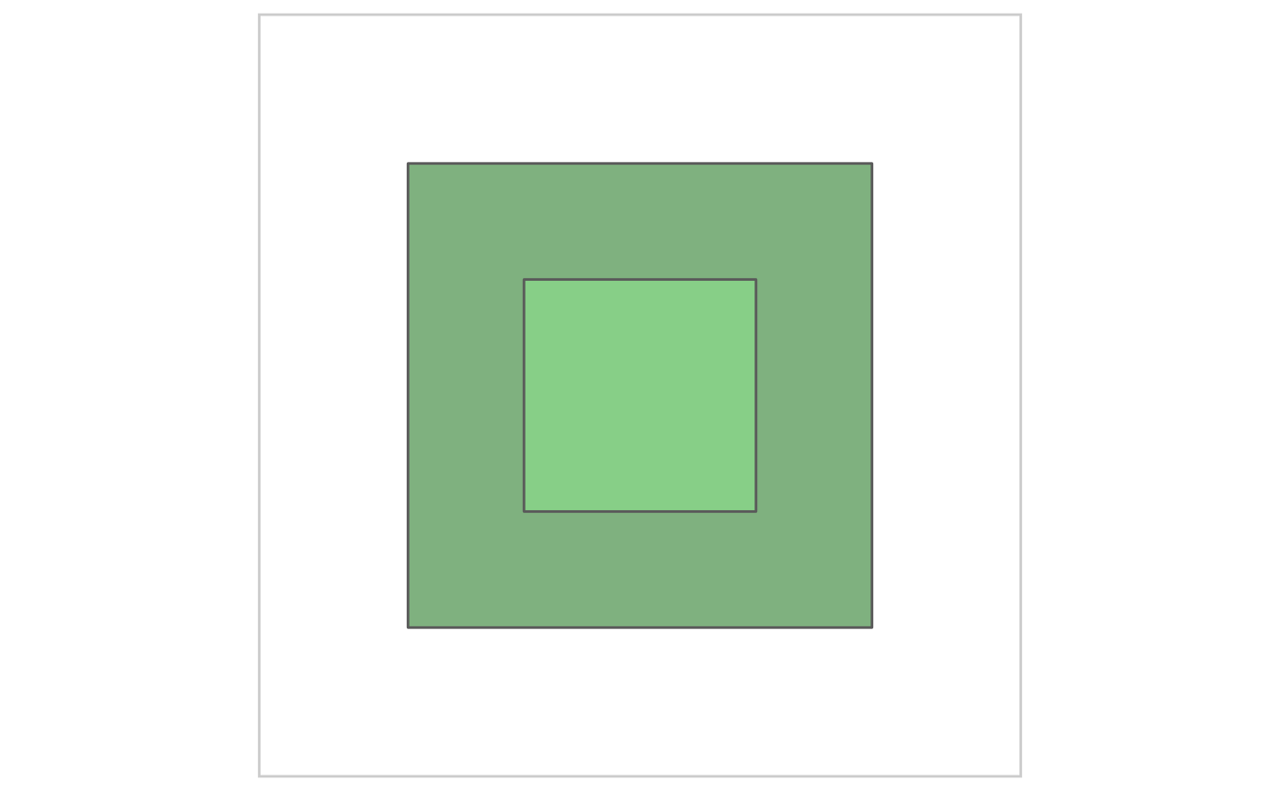
basemap <-
  ggplot2::ggplot() +
  layer_location_data(
    data = bbox_large,
    fill = "darkgreen",
    alpha = 0.5
  ) +
  layer_location_data(
    data = bbox_small,
    fill = "lightgreen",
    alpha = 0.5
  ) +
  layer_neatline(
    data = bbox_large,
    dist = 100,
    unit = "meter",
    color = "gray80"
  )

basemap

small_diamond_sf <-
  st_inscribed_square(x = bbox_small, rotate = 45)

large_diamond_sf <-
  st_scale_rotate(x = bbox_large, scale = 1.25, rotate = 15)

basemap +
  layer_location_data(
    data = small_diamond_sf,
    fill = NA,
    color = "black",
    alpha = 0.1
  ) +
  layer_location_data(
    data = large_diamond_sf,
    fill = NA,
    color = "black",
    alpha = 0.1
  )

center <-
  st_center(x = bbox_large)

dplyr::glimpse(center)
#> List of 5
#>  $ sfc     :sfc_POINT of length 1; first list element:  'XY' num [1:2] -8539713 4757981
#>  $ sf      :Classes 'sf' and 'data.frame':   1 obs. of  3 variables:
#>   ..$ lon     : num -8539713
#>   ..$ lat     : num 4757981
#>   ..$ geometry:sfc_POINT of length 1; first list element:  'XY' num [1:2] -8539713 4757981
#>   ..- attr(*, "sf_column")= chr "geometry"
#>   ..- attr(*, "agr")= Factor w/ 3 levels "constant","aggregate",..: NA NA
#>   .. ..- attr(*, "names")= chr [1:2] "lon" "lat"
#>  $ geometry:sfc_POLYGON of length 1; first list element: List of 1
#>   ..$ : num [1:5, 1:2] -8539914 -8539512 -8539512 -8539914 -8539914 ...
#>   ..- attr(*, "class")= chr [1:3] "XY" "POLYGON" "sfg"
#>  $ x       :Classes 'sf' and 'data.frame':   1 obs. of  1 variable:
#>   ..$ geometry:sfc_POLYGON of length 1; first list element: List of 1
#>   .. ..$ : num [1:5, 1:2] -8539914 -8539512 -8539512 -8539914 -8539914 ...
#>   .. ..- attr(*, "class")= chr [1:3] "XY" "POLYGON" "sfg"
#>   ..- attr(*, "sf_column")= chr "geometry"
#>   ..- attr(*, "agr")= Factor w/ 3 levels "constant","aggregate",..: 
#>   .. ..- attr(*, "names")= chr(0) 
#>  $ crs     :List of 2
#>   ..$ input: chr "EPSG:3857"
#>   ..$ wkt  : chr "PROJCRS[\"WGS 84 / Pseudo-Mercator\",\n    BASEGEOGCRS[\"WGS 84\",\n        DATUM[\"World Geodetic System 1984\"| __truncated__
#>   ..- attr(*, "class")= chr "crs"

bbox_stretched <-
  sf_bbox_expand(
    bbox = bbox_small,
    y_nudge = 50
  )

basemap +
  layer_location_data(
    data = bbox_stretched,
    alpha = 0.1
  )

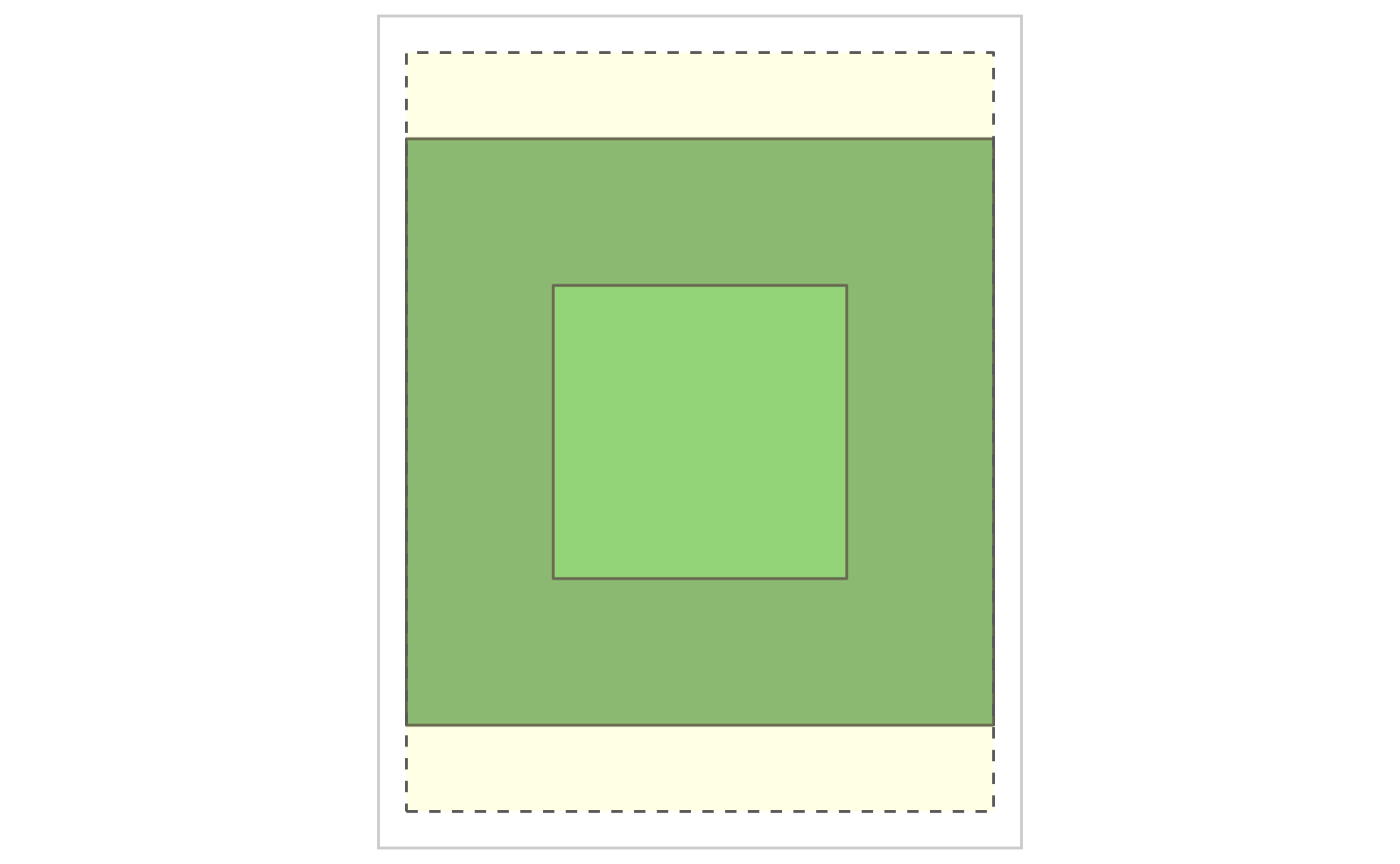
paper_sf <-
  st_bbox_asp(
    x = bbox_large,
    asp = 8.5 / 11,
    class = "sf"
  )

sf::st_geometry(paper_sf) <- "geometry"

basemap +
  layer_location_data(
    data = paper_sf,
    alpha = 0.1,
    fill = "yellow",
    linetype = "dashed"
  )