Set map limits to a simple feature or bounding box with a specified distance buffer, aspect ratio, and panel border
Source:R/layer_neatline.R
layer_neatline.RdSet limits for a map to the bounding box of an x using
ggplot2::coord_sf(). Optionally, adjust the x size by applying a
buffer and/or adjust the aspect ratio of the limiting bounding box to match a
set aspect ratio.
Usage
layer_neatline(
  data = NULL,
  dist = getOption("overedge.dist"),
  diag_ratio = getOption("overedge.diag_ratio"),
  unit = getOption("overedge.unit", default = "meter"),
  asp = getOption("overedge.asp"),
  crs = getOption("overedge.crs"),
  color = "black",
  bgcolor = "white",
  size = 1,
  linetype = "solid",
  expand = FALSE,
  hide_grid = TRUE,
  label_axes = "----",
  ...
)
Arguments
- data
sforbboxclass object- dist
buffer distance in units. Optional.
- diag_ratio
ratio of diagonal distance of area's bounding box used as buffer distance. e.g. if the diagonal distance is 3000 meters and the "diag_ratio = 0.1" a 300 meter will be used. Ignored when
distis provided.- unit
Buffer units; defaults to meter.
- asp
Aspect ratio of width to height as a numeric value (e.g. 0.33) or character (e.g. "1:3"). If numeric,
get_asp()returns the same value without modification.- crs
Coordinate reference system to use for
ggplot2::coord_sf().- color
Color of panel border, Default: 'black'
- bgcolor
Fill color of panel background; defaults to "white". If "none", panel background is set to ggplot2::element_blank()
- size
Size of panel border, Default: 1
- linetype
Line type of panel border, Default: 'solid'
- expand
Default
FALSE.IfTRUE, the function addsggplot2::scale_y_continuous()andggplot2::scale_x_continuous()to expand the map extent to provided parameters.- hide_grid
If
TRUE, hide major grid lines. Default:TRUE- label_axes
A description of which axes to label passed to
ggplot2::coord_sf(); defaults to '----' which hides axes labels.- ...
Additional parameters to pass to
ggplot2::coord_sf().
Value
ggplot2::coord_sf() function with xlim and ylim
parameters
See also
Other layer:
layer_frame(),
layer_icon(),
layer_location_data(),
layer_markers(),
layer_mask(),
layer_scaled()
Examples
nc <- read_sf_path(system.file("shape/nc.shp", package = "sf"))
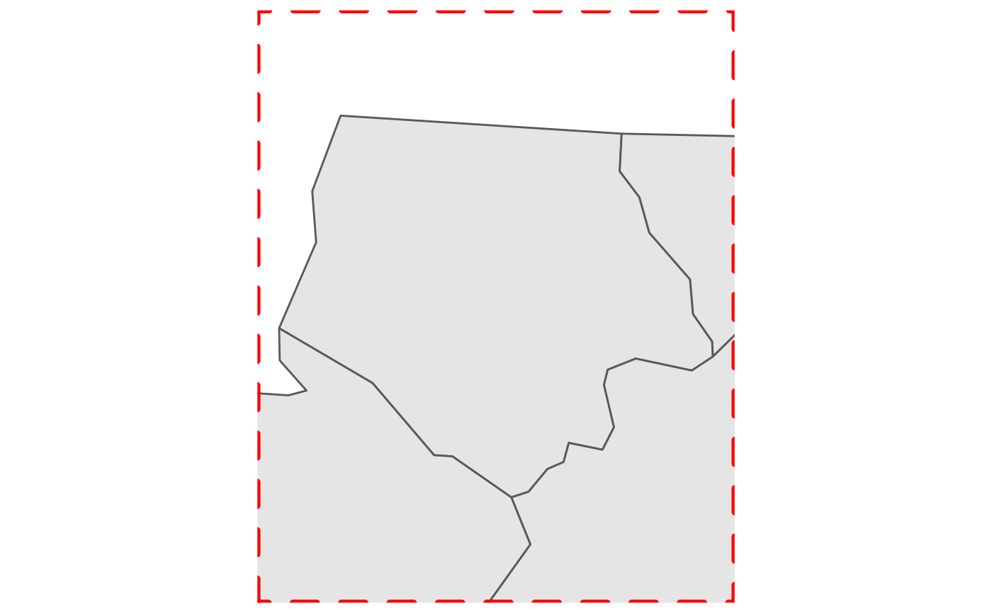
ggplot2::ggplot() +
layer_location_data(data = nc) +
layer_neatline(data = nc[1, ], asp = 1, color = "red", size = 1.5, linetype = "dashed")
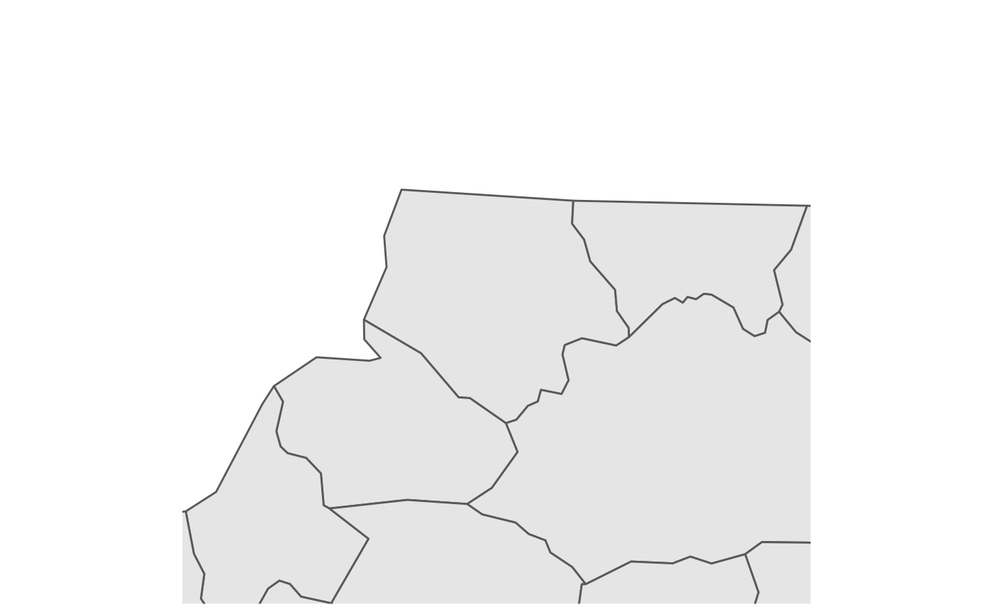
 ggplot2::ggplot() +
layer_location_data(data = nc) +
layer_neatline(data = nc[1, ], dist = 20, unit = "mi", color = "none")
ggplot2::ggplot() +
layer_location_data(data = nc) +
layer_neatline(data = nc[1, ], dist = 20, unit = "mi", color = "none")